Definition of Operational Risk

Operational Risk is an enterprise-wide risk. Operational Risk Management looks across the enterprise in a holistic manner to create a detailed risk profile that can be used by business heads and senior management to run their business more effectively and efficiently.

Basel II defines Operational Risk as losses resulting from inadequate or failed internal processes, people and systems or from external events including legal risk (as fraud constitutes the most significant OR loss events category and a legal issue) but excluding strategic & reputational risks. Thus, all risks other than Credit and Market Risk, come under Operational Risk. Operational Risk is diverse in its scope and includes the risks emanating from all areas of business. It is Complex in causes, sources and its manifestations. Operational Risk is taken not because of financial reward (like credit & market risks), but exists in a normal course of business activity. There are no well established quantitative approaches available for its quantification like Credit & Market Risk.

The Basel Committee has identified the following types of Operational Risks (Event Types) as having the potential to result in substantial losses: 

i. Internal Fraud 

ii. External Fraud 

iii. Employment practices and workplace safety 

iv. Clients, products and business practices 

v. Damage to physical assets 

vi. Business disruption and system failures 

vii. Execution, delivery and process management 

Operational Risk differs from other banking risks in that it is typically not directly taken in return for an expected reward but is implicit in the ordinary course of corporate activity and has the potential to affect the risk management process. ‘Management’ of Operational Risk means the ‘identification, assessment, monitoring & control/mitigation‘ of this risk.

Legal Risk 

A legal risk is a risk that has a legal issue as its source. A legal issue is a set of facts that are assessed under a set of legal norms. Legal risk management focuses on the management of legal risk and the legal management of risk. Legal Risk Management consists of Structural risk management, Compliance risk management, Contractual risk management and Litigation risk management.

Legal risk management process involves the legal and factual context. Identification of legal risks, analysis of legal & factual uncertainty, Legal Risk evaluation both quantitative & qualitative and Risk treatment from both legal & factual risk controls, taking into account the Communication between client, lawyers and non-lawyers. This involves Monitoring and review of legal issues, disputes and cases.

Causes of legal risk materializing

Breakdown of the law enforcement “industry”

Corruption

Political & Occult interests

Exploitation of loopholes in the law

Financial products are not protected neither with copyright, nor licensing. As a result, business may be lost to non-banking institutions.

Impact of Operational Losses

BARINGS PLC – 1995, USD 1.3 Bln – unauthorized trading by Nick Leighson. 

Mizuho Securities – Dec 2005 (USD 250 Mio) – trader error (sold 620 K shares for 1 yen, instead of 1 share for Yen 620K) – shares sold over 4 times the outstanding shares in the company; failures at Mizuho, incl. ―fat finger‖ syndrome, and TSE clearing failures. 

SG – Jan-2008 Euro 4.9 bio net (or 6.3 bio gross of unauthorized profile of Euro 1.4 bio) – unauthorized trades, false hedges, risk measured on net basis, password management, knowledge of controls, weak controls; ―culture of tolerance‖, ignoring warning  signs, incentive structure of traders etc. 

UBS – credit write-downs related to sub-prime exposure of over $ 38 billion. S&P downgraded rating one notch to AA- and may lower further due to ―risk management lapses. Tier 1 ratio would fall to 7% without capital increase and rights issue (an ELEMENT OF OPERATIONAL RISK within this credit risk loss). 

US Mortgage Crisis – non-registration of mortgage loans – instead of registering security interest with local authority, banks did it with a parallel MERS (owned by them) – 64 Mio mortgages under question. 

London Whale – In September 2012, JPMorgan Chase trader Bruno Iksil (nicknamed the London Whale) gambled big on an obscure corner of the credit market—and lost in spectacular fashion. The London Whale not only incurred $6.2 billion in trading losses but allegedly also mismarked some of the losses to cover up their magnitude. His supervisor, Javier Martin-Artajo, was sued by the bank for assisting in the cover-up, JP Morgan Chase has agreed to pay four regulators $920m(£572m) relating to a $6.2bn loss incurred as a result of the “London Whale” trades. The settlement is the third biggest banking fine by US regulators, and the second largest by UK regulators.

UBS – In early September 2011, the Swiss bank UBS announced that it had lost USD $ 2.3 billion dollars, as a result of unauthorized trading performed by Kweku Adoboli, a director of the bank’s Global Synthetic Equities Trading team in London. Britain’s financial regulator has fined UBS $47.5 million for failing to prevent a $2.3 billion loss caused by a former trader.

All these major Losses Raise Importance of Operational Risk Management.

Why Operational Risk Management Needed

• Globalization
• Growth of e-commerce and mobile banking
• Large-scale mergers and acquisitions
• Highly automated technology
• Large volume service providers
• Increased outsourcing
• Very Complex and very large number of products
• Increased business volume
• Increased litigation
• Increased Regulatory fines and penalties
• Loss in reputation
• Huge Loss incurred in business due to operational error

Increased regulatory focus has caused a surge in development by banks in operational risk management and measurement.

Interactions among Credit, Market & Operational Risk

There is a close interaction among Credit, Market and Operational Risk. Consider, for instance, the case of the man responsible for the largest trading loss in British banking history. Kweku Adoboli was a Ghanaian-born British trader at Swiss bank UBS Global Synthetic Equities Trading team in London. On 16 September 2011, it was announced that City of London, Police charged Adoboli with fraud by abuse of position and false accounting dating back to 2008. He was jailed for seven years for fraud over £1.4bn UBS loss after being found guilty of two counts of fraud. He undertook unauthorised trading and 

• Impact: Shares in Swiss bank UBS slumped by 10% following the scandal. All other banking stocks fell. Market Risk increased for all portfolios.
• Credit ratings agency Moody’s downgraded UBS’s rating. Credit Risk also increased because of Operational Risk at UBS.
• UBS were fined £29.7 million in November 2012 for significant failings which prevented them from detecting the unauthorised trading.
• The Financial Conduct Authority (FCA) banned John Christopher Hughes, the Senior Most Trader in ETF Desk in London from performing any function in relation to any regulated activity in the financial services industry for failings related to US$2.3 billion unauthorised trading losses by another trader Kweku Mawuli Adoboli.  The FCA found that Hughes is not a fit and proper person. 
•  The CEO Oswald Grübel had to resign in the wake of the loss and a new CEO, Sergio Ermotti was appointed.

 The Investment Banking Division was reduced in scope and size significantly. It was barred from trading in complex derivatives.

Operational Risk Management Framework (ORMF) and Operational Risk Measurement System (ORMS) 

Operational Risk Management Framework comprises of the organizational structure for management of operational risk, governance structures, policies, procedures and processes and systems used by the organization in identifying, measuring, monitoring, controlling and mitigating operational risk. Banks should develop, implement and maintain a ORMF that is fully integrated into the bank’s overall risk management processes. The Framework for operational risk management chosen by an individual bank will depend on a range of factors, including its nature, size, complexity and risk profile.   A bank with AMA approval must have in place an ORMF that is sufficiently robust to facilitate quantitative estimates of the bank’s Operational Risk Regulatory Capital (ORRC) that is sound, relevant and verifiable.

Operational Risk Management System consists of the mathematical and statistical models, technological support systems, data and validation processes used to measure operational risk to estimate the regulatory capital. ORMS is a subset of ORMF. The regulator must be satisfied that the bank’s ORMF is suitably rigorous and consistent with the complexity of the bank’s business. Where industry risk modelling practices evolve and improve over time, the bank must consider these developments in assessing its own practices. Furthermore, the AMA must play an integral role in the bank’s risk management and decision-making processes and meet the requirements detailed in subsequent paragraphs, including requirements relating to the Board of Directors (Board) and senior management responsibilities. A bank seeking AMA approval must demonstrate the processes it has undertaken to establish an ORMF. The bank will also be required to demonstrate the processes that are undertaken to ensure the continued relevance to the bank’s operations of the operational risk management framework.

Qualitative Standards for the ORMF 

A financial institution must meet the qualitative standards as given below before it is permitted to use an AMA for operational risk capital by regulator.

The bank must have an independent operational risk management function that is responsible for the design and implementation of the bank’s operational risk management framework. The operational risk management function is responsible for codifying firm-level policies and procedures concerning operational risk management and controls; for the design and implementation of the firm’s operational risk measurement methodology; for the design and implementation of a risk-reporting system for operational risk; and for developing strategies to identify, measure, monitor and control/mitigate operational risk. 

There must be regular reporting of operational risk exposures and loss experience to business unit management, senior management, and to the board of directors. The bank must have procedures for taking appropriate action according to the information within the management reports. The bank’s operational risk management system must be well documented. The bank must have a routine in place for ensuring compliance with a documented set of internal policies, controls and procedures concerning the operational risk management system, which must include policies for the treatment of noncompliance issues. 

A bank must have and maintain rigorous procedures for the development, implementation and review of the ORMF. These procedures should ideally include internal validation and external validation of ORMS, and internal audit and external audit of both quantitative and qualitative aspects of entire ORMF. However, at a minimum, the bank must have one of “internal audit” or “external audit” AND one of “internal validation” or “external validation” to qualify for implementation of AMA. The bank will be required to have all four in place before the prudential floors are removed. 

The staff carrying out internal validation and internal auditors should have adequate exposure to handling validation of operational risk models. It should be ensured that the staff of the firms hired for external validation and external audit also have adequate exposure to handling validation of quantitative models in a large financial organisation in addition to possessing necessary qualifications in the relevant areas such as statistics, mathematics, econometrics and information technology, and risk management. 

Qualitative Standards for ORMS 

The ORMS of a bank should be conceptually sound and implemented with integrity. It should also be sufficiently robust to facilitate quantitative estimates of the operational risk capital requirement of the bank. The bank should ensure that the ORMS adopted is implemented consistently across the bank and the ORMS should have a reasonable track record in measuring operational risk. 

The bank’s internal operational risk measurement system must be closely integrated into the day-to-day risk management processes of the bank. This would include ensuring that the output of the ORMS is an integral part of the process of identifying, assessing, monitoring, controlling and mitigating the operational risk of 15 the bank. For example, this output should play a prominent role in risk analysis, managing and reporting, as well as in decision-making, corporate governance and internal capital allocation. Each business line should be able to clearly articulate the drivers of its operational risk and demonstrate how the individual parts of the ORMS are used to supplement its day-to-day decision-making activities.  

A bank should demonstrate, through its internal risk management and decision-making processes that the estimates of the AMA elements produced from internal models do not result in an understatement of risk elements. It should have techniques for allocating operational risk capital to business lines and for creating incentives to improve the management of operational risk, processes and practices throughout the bank. The bank should be able to demonstrate that the allocation will enhance transparency, risk awareness and operational risk management expertise in the bank. 

Quantitative Standards for the ORMS

Given the continuing evolution of approaches for operational risk, Basel II/III framework does not specify any particular approach, methodology, measurement technique or distributional assumptions used to generate the operational risk measure for the purposes of determining the operational risk capital requirement of a bank. 

Operational Risk Management Objectives 

The fundamental goal of operational risk management should be risk prevention. The quantitative measurement of operational risk is of secondary importance. Since complete elimination of operational risk failures is not feasible, the operational risk management framework (ORF) must aim to minimize the potential for loss – through whatever means possible.

The policy aims to achieve the following broad objectives:

• To formally and explicitly define and explain what the words ‘operational risk’ mean to the institution.
• To avoid potential catastrophic losses.
• To enable the institution to anticipate all kinds of risks more effectively, thereby preventing failures from happening.
• To generate a broader understanding of enterprise-wide operational risk issues at all levels and business units of the institution, in addition to the more commonly monitored credit risk and market risk.
• To make the institution less vulnerable to such breakdowns in internal controls and corporate governance as fraud, error, or failure to perform in a timely manner which could cause the interests of the institution to be unduly compromised.
• To identify problem areas in the institution before they become critical.
• To prevent operational mishaps from occurring.
• To establish clarity of people’s roles, responsibilities and accountability.
• To strengthen management oversight at all levels.
• To identify business units in the institution with high volumes, high turnover (i.e., transactions per unit time), high degree of structural change, and highly complex support systems. Such business units are especially susceptible to operational risk.
• To empower business units with the responsibility and accountability of the business risks they assume on a daily basis.
• To provide objective measurements of performance for operational risk management.
• To monitor the danger signs of both income and expense volatilities.
• To effect a change of behaviour within the institution and to enhance the culture of control and compliance within the enterprise.
• To ensure that there is compliance to all risk policies of the institution and to modify risk policies where appropriate.
• To provide objective information so that all services offered by the institution take account of operational risks.
• To ensure that there is a clear, orderly and concise measure of due diligence on all risk-taking and non-risk-taking activities of the institution.
• To provide the executive committee4 regularly with a concise ‘state of the enterprise’report for strategic and planning purposes.

• To define the organization Structure for Operational Risk Management 
• To define the Bank’s Operational Risk strategy and appetite 
• To ensure assignment of roles & responsibility for management of Operational Risk 
• To define the risk identification, assessment and monitoring methodology 
• To facilitate establishment of comprehensive process for detection, reporting and tracking operational loss events 
• To establish training and awareness programs for promoting a risk sensitive culture throughout the Bank 
• To fortify the business & support groups to control and mitigate Operational Risks 
• To ensure compliance with international best practices on Operational Risk Management 

The scope of an operational risk management function within an institution should aim to encompass virtually every aspect of the business process undertaken by the enterprise. The enterprise should manage the Operational Risk arising out of people, process or system inadequacies or that resulting from external events on a pro-active basis. This should be implemented through effective risk identification, assessment and importantly monitoring measures focusing on early-warning indicators. It should be noted that unlike other types of risks, Operational Risk is present in each and every function of a bank. Hence to successfully implement the Operational Risk strategy, this policy lays down the roles and responsibilities of different functions including the business and support departments in managing Operational Risk. The effectiveness of the strategy would depend on creating awareness on Operational Risk across all functions in the Bank.

Two broad categories of operational risk:

Operational strategic risk (‘external’)	Operational failure risk (‘internal’)
Defined as the risk of choosing an inappropriatestrategy in response to external factors such as:politicaltaxationregulationsocietalcompetition	Defined as the risk encountered in the pursuit of aparticular chosen strategy due to:people processtechnologyothers

The goal of operational risk management must be to focus on internal processes (as opposed to external events) since only internal processes are within the control of the firm. The firm’s response to external events is, however, a valid concern for operational risk management.

Operational Risk Measurement

There are 4 methods advised by Basel II for measuring the Operational Risk.

1. Basic Indicator Approach (BIA)

2. The Standard Approach (TSA)

3. The Alternate Standard Approach (ASA)

4. Advanced Measurement Approach (AMA) 

Statistical models for Operational Risk are grouped into two main categories: ‘top-down’ and ‘bottom-up’ methods.

 ‘Top-down’ methods

In the Top-down methods, risk estimation is based on macro data without identifying the individual events or the causes of losses. Therefore, operational risks are measured and covered at a central level, so local business units or branches are not involved in the measurement and allocation process. ‘Top-down’ methods include the Basic Indicator Approach where risk is computed as a certain percentage of the variation of some variable, as, for example, gross income, considered as a proxy for firm performance. This approach is suitable for small banks, that prefer a cheap methodology and easy to implement.

‘Bottom-up’ methods

‘Bottom-up’ methods, instead, use individual events to determine the source and amount of operational risk.  Operational Risk exposures and losses are broken into a series of standardized business units (called business lines) and into a group of OR losses according to the nature of the underlying OR event (called event type); ORs are measured at the level of each business line and then aggregated. These techniques are particularly appropriate for large sized banks and those operating at the international or global level, since they can afford the implementation of sophisticated methods, sensitive to the bank’s risk profile. Methods belonging to this class are grouped into the Standard Approach & Advanced Measurement Approach (AMA). Under the AMA, the regulatory capital requirement will equal the risk measure generated by the bank’s internal operational risk measurement system using the quantitative and qualitative criteria set by the Committee. It is an advanced approach as it allows banks to use external and internal loss data as well as internal expertise.

1. Basic Indicator Approach (BIA)

BIA is the default approach. It is highly unsophisticated and a bank that uses this approach should calculate the capital requirements for covering its exposure to operational risks using Gross Income which is the average over three years of the sum of net interest income and net non-interest income, multiplied by Alpha (α) which is a fixed percentage parameter and set as 15% by Basel Committee. The three-year average is calculated on the basis of the last three twelve-monthly observations at the end of the financial year. When audited figures are not available, business estimates may be used.

If for any given observation, the sum of net interest income and net non-interest income is negative or equal to zero, this figure shall not be taken into account in the calculation of the three-year average. The Gross Income shall be calculated as the sum of positive figures divided by the number of positive figures.

BIA generates a very rough estimation of the impact of the bank‘s exposure to operational risks in terms of capital adequacy requirement. The approach implies that there is a positive correlation between losses due to operational risk exposure and the annual gross income of the whole bank. The higher the income of the bank, the greater the likelihood of large losses linked to its exposure to operational risks. This relationship is of course not necessarily true. A bank‘s annual gross income may very well decrease in its most risky business lines at the same time as its income increases even more in its least risky ones. Moreover, it is doubtful whether changes in net interest income are positively correlated with a bank‘s operational risk exposure, particularly in the case these changes are due to higher or lower interest expenses. Rather we are then more likely to find a negative correlation—if there is any correlation at all. BIA is mainly intended for smaller banks for which operational risk exposures are considered to be of only minor importance. Other banks, i.e. mid-sized and larger banks, are supposed to be more exposed to operational risks.

Advantages : Simplicity 

Shortcomings : Linear relationship with exposure indicator 

▪ Non-specific to business type 

▪ Exposure indicator is distorted with business cycle (lower in downturn, higher in upturn)

2. The Standardised Approach (TSA)

In comparison with the Basic Indicator Approach, The Standardized Approach (TSA) is a more advanced method to determine the capital required for covering operational risk losses.  

In TSA, banks’ activities are divided into eight Business Lines (BL): corporate finance, trading & sales, retail banking, commercial banking, payment & settlement, agency services, asset management, and retail brokerage. The business lines are defined in detail in Appendix1. It is possible that some of these business lines are not being pursued by banks in India departmentally, but are being undertaken through subsidiaries. In such cases, these would be completely omitted from the bank’s operational risk capital charge calculations on solo basis, but included in the assessment of group-wide operational risk capital charge. 

Within each business line, gross income is a broad indicator that serves as a proxy for the scale of business operations and thus the likely scale of operational risk exposure within each of these business lines. The capital charge for each business line is calculated by multiplying gross income by a factor (denoted beta-β) assigned to that business line. Beta serves as a proxy for the industry-wide relationship between the operational risk loss experience for a given business line and the aggregate level of gross income for that business line. It should be noted that in TSA gross income is measured for each business line, not the whole institution, i.e. in corporate finance, the indicator is the gross income generated in the corporate finance business line. However, the sum of the gross income of eight business lines should be equal to the gross income of the institution. 

The total capital charge is calculated as the three-year average of the simple summation of the regulatory capital charges across each of the business lines in each year. The year at the end of which the capital is being calculated will also be one of the three years. In any given year, negative capital charges (resulting from negative gross income) in any business line may offset positive capital charges in other business lines without limit. However, where the aggregate capital charge across all business lines within a given year is negative, then the input to the numerator for that year will be zero. The total capital charge will be expressed as: 

K_TSA = {Σ_{years 1-3} max[Σ(GI_1-8 X β_1-8),0]}/3 

Where, 

K_TSA = the capital charge under TSA 

GI_1-8 = annual gross income in a given year, as defined in the Basic Indicator Approach, for each of the eight business lines (Please see Appendix 2) 

β _1-8 = a fixed percentage, set by the Basel Committee, relating the level of required capital to the level of the gross income for each of the eight business lines. The values of beta are detailed below:

 The value of the betas for TSA :

S.No	Business Line	β Factors
1	Corporate finance (β1)	18%
2	Trading and sales(β2)	18%
3	Payment and settlement(β3)	18%
4	Agency services(β4)	15%
5	Asset management(β5)	12%
6	Retail brokerage(β6)	12%
7	Retail banking(β7)	12%
8	Commercial banking(β8)	15%

QUALIFYING CRITERIA FOR ADOPTING TSA

In order to qualify for use of TSA, a bank must satisfy the regulator that at a minimum, it meets ALL the requirements as given below. 

A. Board of Directors and Senior Management Oversight 

The board of directors and senior management of bank should be actively involved in the oversight of the operational risk management framework. There must be regular reporting of operational risk exposures, including material operational losses, to business unit management, senior management, and to the board of directors. For this purpose operational risk exposures would mean the trends in operational losses observed during last few years in each business line and the bank’s perception of likely operational losses in the near future given its internal controls. The bank must have procedures for taking appropriate action according to the information contained in the management reports. 

B. Quality of Operational Risk Management System 

The bank should have an operational risk management system that is conceptually sound and is implemented with integrity. The operational risk management function is responsible for developing strategies to identify, assess, monitor and control/mitigate operational risk; for preparing firm-level policies and procedures concerning operational risk management and controls; for the design and implementation of the firm’s operational risk assessment methodology; and for the design and implementation of a risk-reporting system for operational risk. 

As part of the bank’s internal operational risk assessment system, the bank must systematically track relevant operational risk data including material losses by business line. In order to qualify for TSA, the bank should have collected operational loss data for different business lines at least for one year and reviewed it at the level of Board at least during last six months. Bank’s internal loss data must be comprehensive in that it captures all material activities and exposures from all appropriate sub-systems and geographic locations. A bank must be able to justify that any activity and exposure excluded would not have a significant impact on the overall risk estimates. Bank may have appropriate de minimis gross loss threshold for internal loss data collection. The appropriate threshold may vary somewhat among banks and within a bank across business lines and / or event types. However, particular thresholds may be broadly consistent with those used by the peer banks. Measuring Operational Risk requires both estimating the probability of an operational loss event and the severity of the loss. Besides, banks are encouraged to have break-up of operational loss data into seven loss events within each business line, as given in Appendix 3. This would facilitate transition to the Advanced Measurement Approach by the bank in due course. Its operational risk assessment system must be closely integrated into the risk management processes of the bank. Its output must be an integral part of the process of monitoring and controlling the bank’s operational risk profile. For instance, this information must play a prominent role in risk reporting, management reporting, and risk analysis. The bank must have techniques for creating incentives to improve the management of operational risk throughout the firm. 

The bank’s operational risk management system must be well documented. The bank must have a routine in place for ensuring compliance with a documented set of internal policies, controls and procedures concerning the operational risk management system, which must include policies for the treatment of non compliance issues. The operational risk management processes and assessment system must be subject to validation and regular independent review which can be carried out by its internal audit department at least annually. These reviews must include both the activities of the business units and of the operational risk management function. 

Moreover, the operational risk assessment system (including the internal validation processes) must be subject to regular review by external auditors (including statutory auditors) and/or supervisors. The bank must develop specific policies and have documented criteria for mapping gross income for current business lines and activities into the standardized framework. The criteria must be reviewed and adjusted for new or changing business activities as appropriate. The bank may get guided by the principles of business line mapping set out in Appendix 4. 

C.  Allocation of Sufficient Resources 

The bank should have sufficient resources (technical/physical and human) in the use of the approach in the major business lines as well as the control and audit areas. 

Verification By Regulator  

A bank may adopt the TSA/ASA (detailed below) once it satisfies the regulator that the aforesaid qualifying criteria are met by the bank. On receipt of application from the bank, along with supporting documents, for migrating to TSA/ASA, the regulator will inter alia examine the compliance to various requirements contained in these guidelines. Such an evaluation would inter alia comprise the following elements: 

• Documentation of the mapping process, 

• Description of the mapping criteria, 

• Explanation of the mapping of new types of activities, 

• Structure of responsibilities and reporting, 

• Description of the risk management process for operational risk, and 

• Integrity of the operational risk loss data for each business line. 

Advantages : Fairly simple

▪ Specific to business type 

Shortcomings : Linear relationship with risk driver 

▪ Exposure indicator is distorted with business cycle (lower in downturn, higher in upturn)

3. ALTERNATIVE STANDARDISED APPROACH 

The ASA is a special variant of TSA. A bank can use the ASA provided the bank is able to satisfy the regulator that this alternative approach provides an improved basis for risk management. Once a bank has been allowed to use the ASA, it will not be allowed to revert to use of TSA without the permission of the regulator.

Under the ASA, the operational risk capital charge/methodology is the same as for TSA except for two business lines — Retail Banking and Commercial Banking. For these business lines, loans and advances — multiplied by a fixed factor ‘m’ — replaces gross income as the exposure indicator. The betas for retail and commercial banking are unchanged from TSA. 

For instance, the ASA operational risk capital charge for retail banking can be expressed as: 

KRB = B₇ x m x LArB 

where KRB = the capital charge for the retail banking business line B7 = the beta for the retail banking business line.

LArB = total outstanding retail loans and advances (non-risk weighted and gross of provisions), averaged over the past 12 quarters; and 

m = the fixed factor 0.035. 

Overall capital charge under ASA will be calculated as under: 

K_ASA = {Σyears 1-3 max[Σ(GI_1-6 x β1-6),0]} / 3 + (β₇ x m x LArB) + (β₈ x m x LAcB) 

Where 

LArB = total outstanding retail loans and advances (non-risk weighted and gross of provisions), averaged over the past 12 quarters; and 

LAcB = total outstanding commercial banking loans and advances (non-risk weighted and gross of provisions), averaged over the past 12 quarters; and 

m = 0.035 (for both retail and commercial banking) 

For the purposes of the ASA, total loans and advances in the retail banking business line consists of the total drawn amounts in the following credit portfolios: retail, SMEs treated as retail, and purchased retail receivables. For commercial banking, total loans and advances consists of the drawn amounts in the following credit portfolios: corporate, sovereign, bank, specialised lending, SMEs treated as corporate and purchased corporate receivables. The book value of securities held for the purpose of interest income such as in HTM and AFS should also be included. 

Under the ASA, banks may aggregate retail and commercial banking (if they wish to) using a beta of 15%. Similarly, those banks that are unable to disaggregate their gross income into the other six business lines can aggregate the total gross income for these six business lines using a beta of 18%. As under TSA, the total capital charge for the ASA is calculated as the simple summation of the regulatory capital charges across each of the eight business lines. 

QUALIFYING CRITERIA 

In addition to the general requirements for applying the standardized approach, a bank opting for ASA should also satisfy the following additional criteria: 

• The bank must be overwhelmingly active in retail and/or commercial banking activities, which must account for at least 90% of its income indicator; and 

• the bank must be able to demonstrate that a significant proportion of its retail and/or commercial banking activities comprise loans associated with a high probability of default, and that the alternative standardised approach provides an improved basis for assessing the operational risk. 

CALCULATION OF CAPITAL CHARGE FOR OPERATIONAL RISK 

Once the bank has calculated the capital charge for operational risk under TSA/ASA, it has to multiply this with (100÷9) and arrive at the notional risk weighted asset (RWA) for operational risk. The RWA for operational risk will be aggregated with the RWA for the credit risk and the minimum capital requirement (Tier 1 and Tier 2) for credit and operational risk will be calculated. The total of eligible capital (Tier 1 and Tier 2) will be divided by the total RWA (credit risk + operational risk + market risk) to compute CRAR for the bank as a whole. 

Mapping of Business Lines Appendix 1

Level 1	Level 2	Activity Groups
Corporate Finance	Corporate Finance	Mergers and acquisitions, underwriting, privatisations, securitisation, research, debt (government, high yield), equity, syndications, IPO, secondary private placements Note: The Gross Income arising from advisory, on-balance sheet and off-balance sheet activities of banks connected with the above areas would be reckoned under this business line. GI related to financial assistance extended for mergers and acquisitions, wherever permitted as per existing regulatory guidelines, will be reported here.
	Government Finance
	Merchant Banking
	Advisory Services
Trading & Sales	Sales	Fixed income, equity, foreign exchanges, credit products, funding, own position securities, lending and repos, brokerage, debt, prime brokerage and sale of Government bonds to retail investors. Note: GI from cross-selling of various products of the subsidiaries of the bank or other financial institutions, income from derivatives transactions, call money lending transactions, short sale of securities, purchase and sale of foreign currency, should also be reported here.
	Market Making
	Proprietary Positions
	Treasury
Payment and Settlement* *Payment and settlement losses related to a bank’s own activities would be incorporated in the loss experience of the affected business line.	External Clients	Payments and collections, inter-bank funds transfer, clearing and settlement
Agency Services	Custody	Escrow, securities lending (customers) corporate actions, depository services
	Corporate Agency	Issuer and paying agents
	Corporate Trust	Debenture trustee
Asset Management	Discretionary Fund Management	Pooled, segregated, retail, institutional, closed, open, private equity
	Non-Discretionary Fund Management	Pooled, segregated, retail, institutional, closed, open
Retail Brokerage	Retail Brokerage#	Execution and full service
Retail Banking	Retail Banking	Retail lending including trade finance, cash credit etc. as defined under Basel II and also covering non fund based and bill of exchange facilities to retail customers, housing loans, loans against shares, banking services, trust and estates, retail deposits, intra bank fund transfer on behalf of retail customers.
	Private Banking	Private lending (personal loans) and private/bulk deposits, banking services, trust and estates, investment advice
	Card Services	Merchant/commercial/corporate cards, private labels and retail
Commercial Banking	Commercial Banking	Project finance, corporate loans, cash credit loans, real estate, export and import finance, trade finance, factoring, leasing, lending, guarantees including deferred payment and performance guarantees, LCs, bills of exchange, take-out finance, interbank lending other than in call money and notice money market.

Definition of Gross Income Appendix 2

Gross income is defined as “Net interest income” plus “net non-interest income”. It is intended that this measure should: 

i) be gross of any provisions (e.g. for unpaid interest) and write-offs made during the year; 

ii) be gross of operating expenses, including fees paid to outsourcing service providers, in addition to fees paid for services that are outsourced, fees received by banks that provide outsourcing services shall be included in the definition of gross income; 

iii) exclude reversal during the year in respect of provisions and write-offs made during the previous year(s); 

iv) exclude income recognised from the disposal of items of movable and immovable property; 

v) exclude realised profits / losses from the sale of securities in the “held to maturity” category; 

vi) exclude income from legal settlements in favour of the bank; 

vii) exclude other extraordinary or irregular items of income and expenditure; and 

viii) exclude income derived from insurance activities (i.e. income derived by writing insurance policies) and insurance claims in favour of the bank. 

The above definition is summarized in the following equation: 

Gross Income = Net profit (+) Provisions & contingencies (+) Operating expenses (Schedule 16 of Balance Sheet) (-) items (iii) to (viii) of paragraph above. 

Advantages : Fairly simple 

▪ Specific to business type 

▪ More stable prediction through business cycle 

Shortcomings : Linear relationship with exposure indicators

Detailed Loss Event Type Classification Appendix 3 

Event-Type Category (Level 1)	Definition	Categories (Level 2)	Activity Examples (Level 3)
Internal fraud	Losses due to acts of a type intended to defraud, misappropriate property or circumvent regulations, the law or company policy, excluding diversity/ discrimination events, which involves at least one internal party	Unauthorized Activity	Transactions not reported (intentional)
			Transaction type unauthorized (with monetary loss)
			Mismarking of position (intentional)
		Theft and Fraud	Fraud / credit fraud / worthless deposits
			Theft / extortion / embezzlement / robbery
			Misappropriation of assets
			Malicious destruction of assets
			Forgery
			Kite flying
			Smuggling
			Account take-over / impersonation / etc.
			Tax non-compliance / evasion (wilful)
			Bribes / kickbacks
			Insider trading (not on firm’s account)
External fraud	Losses due to acts of a type intended to defraud, misappropriate property or circumvent the law, by a third party	Theft and Fraud	Theft/Robbery
			Forgery
			Kite flying
		Systems Security	Hacking damage
			Theft of information (with monetary loss)
Employment Practices and Workplace Safety	Losses arising from acts inconsistent with employment, health or safety laws or agreements, from payment of personal injury claims, or from diversity / discrimination events	Employee Relations	Compensation, benefit, termination issues
			Organised labour activity
		Safe Environment	General liability (slips and falls, etc.)
			Employee health & safety rules events
			Workers compensation
		Diversity & Discrimination	All discrimination types

Event-Type Category (Level 1)	Definition	Categories (Level 2)	Activity Examples (Level 3)
Clients, Products & Business Practices	Losses arising from an unintentional or negligent failure to meet a professional obligation to specific clients (including fiduciary and suitability requirements), or from the nature or design of a product.	Suitability, Disclosure & Fiduciary	Fiduciary breaches / guideline violations
			Suitability / disclosure issues (KYC, etc.)
			Retail customer disclosure violations
			Breach of privacy
			Aggressive sales
			Account churning
			Misuse of confidential information
			Lender liability
		Improper Business or Market Practices	Antitrust
			Improper trade / market practices
			Market manipulation
			Insider trading (on firm’s account)
			Unlicensed activity
			Money laundering
		Product Flaws	Product defects (unauthorised, etc.)
			Model errors
		Selection, Sponsorship & Exposure	Failure to investigate client per guidelines
			Exceeding client exposure limits
		Advisory Activities	Disputes over performance of advisory activities
Damage to Physical Assets	Losses arising from loss or damage to physical assets from natural disaster or other events.	Disasters and other events	Natural disaster losses
			Human losses from external sources (terrorism, vandalism)
Business disruption and system failures	Losses arising from disruption of business or system failures	Systems	Hardware
			Software
			Telecommunications
			Utility outage / disruptions

Event-Type Category (Level 1)	Definition	Categories (Level 2)	Activity Examples (Level 3)
Execution, Delivery & Process Management	Losses from failed transaction processing or process management, from relations with trade counterparties and vendors	Transaction Capture, Execution & Maintenance	Miscommunication
			Data entry, maintenance or loading
			Missed deadline or responsibility
			Model / system misoperation
			Accounting error/entity attribution
			Other task misperformance
			Delivery failure
			Collateral management failure
			Reference Data Maintenance
		Monitoring and Reporting	Failed mandatory reporting obligation
			Inaccurate external report (loss incurred)
		Customer Intake and Documentation	Client permissions / disclaimers missing
			Legal documents missing / incomplete
		Customer / Client Account Management	Unapproved access given to accounts
			Incorrect client records (loss incurred)
			Negligent loss or damage of client assets
		Trade Counterparties	Non-client counterparty misperformance
			Misc. non-client counterparty disputes
		Vendors & Suppliers	Outsourcing
			Vendor disputes

Principles for Business Line Mapping Appendix 4

(a) All activities must be mapped into the eight level 1 business lines in a mutually exclusive and jointly exhaustive manner. 

(b) Any banking or non-banking activity which cannot be readily mapped into the business line framework, but which represents an ancillary function to an activity included in the framework, must be allocated to the business line it supports. If more than one business line is supported through the ancillary activity, an objective mapping criteria must be used. 

(c) When mapping gross income, if an activity cannot be mapped into a particular business line then the business line yielding the highest charge must be used. The same business line equally applies to any associated ancillary activity. 

(d) Banks may use internal pricing methods to allocate gross income between business lines provided that total gross income for the bank (as would be recorded under the Basic Indicator Approach) still equals the sum of gross income for the eight business lines. 

(e) The mapping of activities into business lines for operational risk capital purposes must be consistent with the definitions of business lines used for regulatory capital calculations in other risk categories, i.e. credit and market risk. Any deviations from this principle must be clearly motivated and documented. 

(f) The mapping process used must be clearly documented. In particular, written business line definitions must be clear and detailed enough to allow third parties to replicate the business line mapping. Documentation must, among other things, clearly motivate any exceptions or overrides and be kept on record. 

(g) Processes must be in place to define the mapping of any new activities or products. 

(h) Senior management is responsible for the mapping policy (which is subject to the approval by the board of directors).

 (i) The mapping process to business lines must be subject to independent review. 

Supplementary Business Line Mapping Guidelines 

There are a variety of valid approaches that banks can use to map their activities to the eight business lines, provided the approach used meets the business line mapping principles. The following is an example of one possible approach that could be used by a bank to map its gross income: 

1. Gross income for retail banking consists of net interest income on loans and advances to retail customers and SMEs treated as retail, plus fees related to traditional retail activities, net income from swaps and derivatives held to hedge the retail banking book, and income on purchased retail receivables. To calculate net interest income for retail banking, a bank takes the interest earned on its loans and advances to retail customers less the weighted average cost of funding of the loans (from whatever source). 

2. Similarly, gross income for commercial banking consists of the net interest income on loans and advances to corporate (plus SMEs treated as corporate), interbank and sovereign customers and income on purchased corporate receivables, plus fees related to traditional commercial banking activities including commitments, guarantees, bills of exchange, net income (e.g. from coupons and dividends) on securities held in the banking book, and profits/losses on swaps and derivatives held to hedge the commercial banking book. Again, the calculation of net interest income is based on interest earned on loans and advances to corporate, interbank and sovereign customers less the weighted average cost of funding for these loans (from whatever source). 

3. For trading and sales, gross income consists of profits/losses on instruments held for trading purposes (i.e. in the mark-to-market book), net of funding cost, plus fees from wholesale broking. 

4. For the other five business lines, gross income consists primarily of the net fees/commissions earned in each of these businesses. Payment and settlement consists of fees to cover provision of payment/settlement facilities for wholesale counterparties. Asset management is management of assets on behalf of others. 

4. Advanced Measurement Approach

Paragraph 667 of the Basel II Framework states that “Given the continuing evolution of analytical approaches for operational risk, the Committee is not specifying the approach or distributional assumptions used to generate the operational risk measure for regulatory capital purposes. However, a bank must be able to demonstrate that its approach captures potentially severe ’tail’ loss events. Whatever approach is used, a bank must demonstrate that its operational risk measure meets a soundness standard comparable to that of the internal ratings-based approach for credit risk (i.e. comparable to a one year holding period and a 99.9th percentile confidence interval).” Basel III has not touched the Operational Risk.

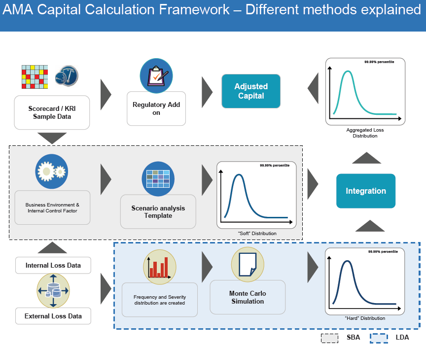
The Advanced Measurement Approach allows a bank to internally develop its own risk measurement model. The rules under advanced measurement approach requires that a bank’s operational loss data captures the operational risks to which the firm is exposed to. The model must include credible, transparent, systematic and verifiable approaches for weighting internal operational loss data, external operational loss data, scenario analysis and BEICFs.

The Four Data Elements

(1) Internal Data

The internal loss data are considered the most important input to the model and are thought to reflect the bank’s risk profile most accurately. The data are exclusively used in calibrating the frequency parameters and are used in combination with external data to calibrate the severity distribution. Also frequency dependencies are analyzed using internal data.

While the Basel II Framework provides flexibility in the way a bank combines and uses the four data elements in its operational risk management framework (ORMF), regulators expect that the inputs to the AMA model are based on data that represent or the bank’s business risk profile and risk management practices. ILD is the only component of the AMA model that records a bank’s actual loss experience. Supervisors expect ILD to be used in the operational risk measurement system (ORMS) to assist in the estimation of loss frequencies; to inform the severity distribution(s) to the extent possible; and to serve as an input into scenario analysis as it provides a foundation for the bank’s scenarios within its own risk profile. The Committee has observed that many banks have limited high severity internal loss events to inform the tail of the distribution(s) for their capital charge modeling. It is therefore necessary to consider the impact of relevant ED and/or scenarios for producing meaningful estimates of capital requirements.

(2) External Data

External data can be used to enrich the scarce internal data. They can also be used to modify parameters derived from internal data, or as input in scenarios and for benchmarking. Even though external data do not fully reflect the bank’s risk profile, and are generally more heavy tailed than internal data, external data can still be more reliable for calibrating the tail distribution than internal. ED provides information on large actual losses that have not been experienced by the bank, and is thus a natural complement to ILD in modeling loss severity. Supervisors expect ED to be used in the estimation of loss severity as ED contains valuable information to inform the tail of the loss distribution(s). ED is also an essential input into scenario analysis as it provides information on the size of losses experienced in the industry. Note that ED may have additional uses beyond providing information on large losses for modeling purposes. For example, ED may be useful in assessing the riskiness of new business lines, in benchmarking analysis on recovery performance, and in estimating

competitors’ loss experience.

While the ED can be a useful input into the capital model, external losses may not fit a particular bank’s risk profile due to reporting bias. Reporting bias is inherent in publicly sourced ED and therefore focuses on larger, more remarkable losses. A bank should address these biases in their methodology to incorporate ED into the capital model. As ED may not necessarily fit a particular bank’s risk profile, a bank should have a defined process to assess relevancy and to scale the loss amounts as appropriate. A data filtering process involves the selection of relevant ED based on specific criteria and is necessary to ensure that the ED being used is relevant and consistent with the risk profile of the bank. To avoid bias in parameter estimates, the filtering process should result in consistent selection of data regardless of loss amount. If a bank

permits exceptions to its selection process, the bank should have a policy providing criteria for exceptions and documentation supporting the rationale for any exceptions. A data scaling process involves the adjustment of loss amounts reported in external data to fit a bank’s business activities and risk profile. Any scaling process should be systematic, statistically supported, and should provide output that is consistent with the bank’s risk profile.

To the extent that little or no relevant ED exists for a bank, supervisors would expect the model to rely more heavily on the other data elements. Limitations in relevant ED most frequently arise for banks operating in distinct geographic regions

or in specialised business lines.

(3) Scenario Analysis

Scenarios are used as a complement to historical loss data and are used where data are scarce. Scenario data are forward looking, unlike external and internal data, and include events that have not yet occurred. Scenario analysis is inherently biased, such as anchoring, availability and motivational biases.

A robust scenario analysis framework is an important element of the ORMF. This scenario process will necessarily be

informed by relevant ILD, ED and suitable measures of BEICFs. While there are a variety of integrated scenario approaches, the level of influence of scenario data within these models differs significantly across banks. The scenario process is qualitative by nature and therefore, the outputs from a scenario process necessarily contain significant

uncertainties. This uncertainty, together with the uncertainty from the other elements, should be reflected in the output

of the model producing a range for the capital requirements estimate. Thus, scenario uncertainties provide a mechanism for estimating an appropriate level of conservatism in the choice of the final regulatory capital charge. Because quantifying the uncertainty arising from scenario biases continuous to pose significant challenges, a bank should closely observe the integrity of the modelling process and engage closely with the relevant supervisor.

Scenario data provides a forward-looking view of potential operational risk exposures. A robust governance framework

surrounding the scenario process is essential to ensure the integrity and consistency of the estimates produced. An established scenario framework will have the following features:

(a) A clearly defined and repeatable process;

(b) Good quality background preparation of the participants in the scenario generation process; 

(c) Qualified and experienced facilitators with consistency in the facilitation process;

 (d) The appropriate representatives of the business, subject matter experts and the corporate operational risk management function as participants involved in the process; 

(e) A structured process for the selection of data used in developing scenario estimates;

(f) High quality documentation which provides clear reasoning and evidence supporting the scenario output; 

(g) A robust independent challenge process and oversight by the corporate operational risk management function to ensure the appropriateness of scenario estimates; 

(h) A process that is responsive to changes in both the internal and external environment; and 

(j) Mechanisms for mitigating biases inherent in scenario processes. Such biases include anchoring, availability and motivational biases.

(4) Business Environment & Internal Control Factors (BEICF)

The fourth element and input in an AMA model are the Business Environment and Internal Control Factors (BEICFs). LDA models mainly depend on historical loss data which are backward looking. Therefore it is necessary with the ability to make continuous qualitative adjustments to the model that reflects ongoing changes in business environment and risk exposure.

There are several ways these adjustments can be made and they can vary a lot depending on institution and relevant information collecting process. BEICFs are operational risk management indicators that provide forward-looking assessments of business risk factors as well as a bank’s internal control environment. However, incorporating BEICFs directly into the capital model poses challenges, given the subjectivity and structure of BEICF tools. Banks continue

to investigate and refine measures of BEICFs and explore methods for incorporating them into the capital model. BEICFs are commonly used as an indirect input into the quantification framework and as an ex-post adjustment to model output. Ex-post adjustments serve as an important link between the risk management and risk measurement processes and may

result in an increase or decrease in the AMA capital charge at the group-wide or business-line level. Given the subjective nature of BEICF adjustments, a bank should have clear policy guidelines that limit the magnitude of either positive or negative adjustments. It should also have a policy to handle situations where the adjustments actually exceed these limits based on the current BEICFs. BEICF adjustments should be well-supported and the level of supervisory scrutiny will increase with the size of the adjustment. Over time, the direction and magnitude of adjustments should be compared to ILD, conditions in the business environment and changes in the effectiveness of controls to ensure appropriateness. BEICFs should, at a minimum, be used as an input in the scenario analysis process.

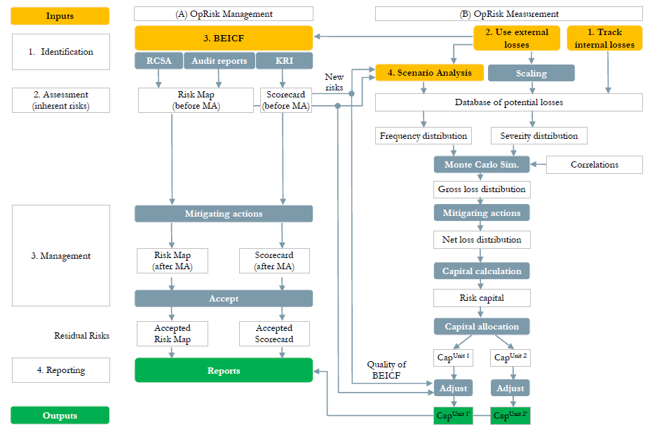
ORM FRAMEWORK IMPLEMENTATION

Operational risk is now implemented through a framework as it touches all aspects of bank. Assessment of operational risk in all material products, processes and systems involves consideration of external and internal factors. The tools include: audit findings, internal loss data collection and analysis, external data collection and analysis, risk assessment, business process mapping, risk and performance indicators, scenario analysis, measurement, comparative analysis (e.g. frequency and severity data with results of RCSA).Example of ORM Framework is given below.

IDENTIFICATION 

Start loss collection infrastructure (internal losses, external losses) 

describe potential losses by structured info 

– preventive measures for high risk areas

– disseminate information via internal communication channels (e.g. e-mail) 

ASSESSMENT

Find quantifiable means to track OR; 

Create Reporting mechanism 

Involve business units 

Invest in automated data gathering & workflow technologies 

MEASUREMENT 

Developing& refining modeling approach

Create Operational Risk Data Library

Technology Development

Implement advanced tools – risk indicators, – scenario analyses, – business process analyses 

INTEGRATED MANAGEMENT 

– Integrate OR exposure data into management process; 

-Engage senior management  

-Manage Exposures 

-Invest in Processes 

Source: IFC: OpsRisk Training

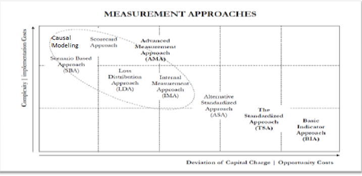
There are mainly five basic methods which are used under AMA:

• Internal Measurement Approach (IMA)
• Loss Distribution Approach (LDA),
• Scorecard Approach (SCA)
• Scenario Based approach (SBA) 
• Causal Modeling.

The last one is a dynamic simulation of operational processes, with outputs in form of operational losses, built by taking all relevant causal drivers into account. Scenario based analysis, as its name already tells, is a method which evaluates operational risk through scenarios. When using Scorecards a questionnaire is used to get information on the risk controls and drivers. These three models are future oriented, thus able to respond quickly to changes in the business environment.

Loss distribution approach is based on realized historical losses, so it is strongly past oriented. In this method the distribution of the yearly losses is determined, and capital is calculated by taking its 99.9% confidence level. This is the Value at Risk (VaR) of the operational losses.

(1) Internal Measurement Approach

Majority of the banks that adopt AMA will at an initial phase be likely to use a simplified variant referred to as the internal measurement approach (IMA). Approach based on linear proxy between expected and unexpected losses. 

Parameters

Parameters

γ = proxy parameter between EL and UL.

PE = probability of loss event during1 year horizon.

LGE = average loss given that an event occurs

EI = exposure indicator to capture the scale of activities for business line i/event type j

LE = single loss event

NE = number of single loss events

Exposure indicators 

▪ Number of transactions

▪ Total turnover of operations 

▪ Average volume of transactions 

▪ Gross income of operations

SOURCES: 1. Working Paper on the Regulatory Treatment of Operational Risk BCBS, 2001.

2. Carol Alexander. Operational Risk: Regulation, Analysis and Management, Pearson Education, 2003, p.148

The required capital for each combination of business line / event type is as follows:

Required Capital = γ *EL = γ * (EI * PE* LGE) (1.1)

where EL = expected average annual loss amount =(EI * PE* LGE).EL is derived from the bank’s own loss data based on the collection of internal data.

As IMA is an alternative under the AMA, the required capital for event type i for business line j ,calculated under the IMA is equal to the Unexpected Loss ULij (tail of the distribution) measured with the holding period and the confidence interval determined by the regulators. ULij is determined either on the basis of actual distribution or theoretically. Furthermore, in order to reflect appropriately the characteristics of Low Frequency High Severity (LFHS) operational risk, an adjustment factor (1+A/√ n) has been incorporated as follows.

Required Capital = λ * EL * (1+A/√ n) (1.2)

where λ denotes a constant determined for each business line, A is a constant for each business line / event type combination and n denotes the number of events. λ is a constant determined based on the holding period and confidence interval specified by the regulators.

The characteristics of the IMA formula (1-2) discussed so far are summarised below.

− It is based on the linear formula EI * PE * LGE (= EL).

− Non-linearity is incorporated through multiplication by the inverse of the square root of the number of events — in order to incorporate the characteristic that risk is higher for the same EL in the case of low-frequency.

− The level of severity is differentiated between event types — in order to incorporate the characteristic that risk is higher for the same EL in the case of high-severity.

− Exposure Indicator is not explicitly shown

− Under the Foundation Model, it is possible to set the floor at a different level from other methods under the AMA because the parameters A and λ can be commonly determined on a global basis, which would negate the necessity for model validation for each bank in the actual implementation of the regulatory framework.

(2) Loss Distribution Approach

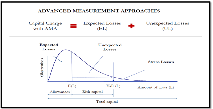
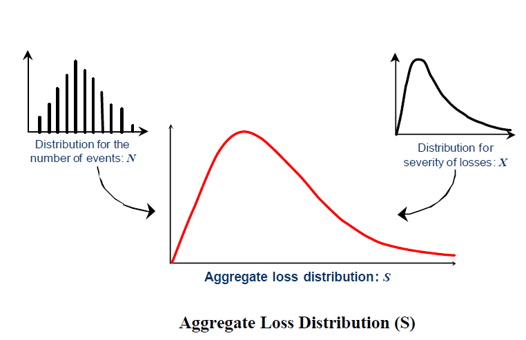
Most of the banks have adopted the Loss distribution Approach (LDA) which is based on historical losses, where frequency and severity of operational losses for each risk cell (in the matrix of eight business lines times seven event types) are estimated over a one year period. Then the capital is estimated using the 99.9% confidence level of the  distribution for the total annual loss in the bank. The LDA has one very important advantage. In the LDA the whole loss distribution is simulated, for each risk type and line of business and this allows the use of aggregation methods that are more appropriate than the aggregation methods that are admissible with the IMA. Unexpected Loss is the difference between VAR and Expected Loss, as Figure 1 shows. This is the amount of capital that the institution should establish to cover unexpected losses for operational risk corresponding to the desired confidence level.

As the statistical distribution of operational losses experienced by different types of business lines across different loss event types exhibit different properties, the bank must map its Operational Risk Categories (ORCs), a business unit or division to various combinations of loss event types and business lines to the loss events types given in Appendix 2 and business lines given in Appendix 3. More specifically, the operational risk losses are characterised by Low Frequency High Severity (LFHS), High Frequency High Severity (HFHS), Low Frequency Low Severity (LFLS) and High Frequency Low Severity (HFLS) events. Modeling of these events require application of specific statistical distributions depending upon the relative proportion of LFHS and HFLS and HFHS events and their behaviour. A separate risk measure consistent with the statistical nature of the underlying distribution of losses should be generated for each recognised combination of business line and loss event type, which in turn may be aggregated to compute the enterprise level operational risk VaR for the purpose of obtaining the operational risk capital charge. As the accuracy of the operational risk measure would, to a great extent, depend upon the correct identification of the underlying distribution, banks need to apply robust statistical techniques to test the reasonableness of the assumptions about the underlying distributions. 

As such, bank should calculate its regulatory operational risk capital requirement as the sum of expected loss (EL) and unexpected loss (UL). Banks should endeavour to account for EL by means of provisions to the extent considered appropriate by them, and the balance through holding capital. This means that if expected loss has been fully provided for in the books of account through debit to profit and loss account, the same can be deducted from the total regulatory capital requirement measured under as per the AMA model as sum of EL and UL. In other words, in such a case, the operational risk capital will be required only for unexpected part of losses. If the provisions held against operational losses exceed the EL, the excess would be eligible for inclusion in Tier II capital subject to the limit of 1.25% of risk weighted assets. The provisions made by banks against identified operational risk loss events which have materialized but the loss is yet to be reflected in the Profit and Loss Account, would be over and above the capital plus provisions required by the banks against expected and unexpected losses measured under the AMA.

A well accepted practice followed by the industry is to model the frequency and severity distributions of operational losses separately and then combine these to calculate the aggregate loss distribution. There is no specific approach or distributional assumptions used to generate the operational risk measure for regulatory capital purposes. However, a bank must be able to demonstrate that its approach captures potentially severe ‘tail’ loss events. 

Distributional assumptions underpin most, if not all, operational risk modeling approaches and are generally made for both operational risk loss severity and the frequency of operational risk loss events. One of the considerations in a bank’s choice of distributions is the existence and size of the threshold above which data are captured and modeled. Threshold simply means, the cut-off limit beyond which no operational losses will be captured and reported. So, if a Bank keeps the Threshold as $10000, then all losses above 10000 dollar only will be captured and reported.  Modeling of operational risk exposures is still relatively new and a common view of appropriate severity distributional assumptions is yet to emerge. The severity of operational risk loss data tends to be heavy-tailed and methodologies for modeling operational risk must be able to capture this attribute. However, a bank’s choice of distribution will have a significant impact on operational risk capital, as will the statistical method used for fitting that distribution. Similarly, a bank’s choice of data threshold may significantly impact the appropriateness of the chosen distributions and/or its estimation method, and consequently the bank’s operational risk capital.

Severity Distribution Model for AMA

Normally, the severity and frequency distributions are modeled separately. For estimating severity distributions, range of distributions exists. AMA may use more than one approach to estimate severity of the body, tail and entire distribution.  The models are used for modeling the severity of the scenario data across all ORCs, regardless of its business, size and complexity. May use more than one approach to estimate severity of the body, tail and entire distribution. First, it is unlikely that the internal and external loss data are drawn from the same underlying severity distribution. Second, there is a general recognition that a single parametric distribution is inadequate to capture the probabilistic behavior of severity over its range. It is generally believed that the severity distribution for the extreme losses behaves differently and is better captured by heavy-tail or fat-tail parametric distributions. 

1. Lognormal Distribution – Light Tailed
2. Weibull Distribution – Light Tailed
3. Gamma Distribution – Light Tailed
4. Exponential Distribution – Light Tailed
5. Log Gamma Distribution – Fat Tailed
6. Pareto Distribution – Fat Tailed
7. Generalised Pareto Distribution – Fat Tailed
8. Burr and Log-Logistic Distribution – Fat Tailed

LFHS & HFHS events are usually the main drivers of risk estimates used in AMA models. Dependencies between such tail events should be studied with great care. Given the different nature of tail and body events, different quantitative & qualitative tools could be necessary to determine and estimate the impact that the underlying dependency structures will have on capital. Due to being heavy tailed, the severity distributions have greater role in influencing the regulatory capital number than the frequency distributions. Banks should document the process of selection of the distribution to represent both severity and frequency. 

Frequency Distribution Model for AMA

To find out the frequency of Operational losses, i.e, number of events that occur within a given time period.

1. Poisson Distribution
2. Negative Binomial Distribution. 
3. Binomial Distribution

The main difficulty of the procedure described above, however, lies in the “aggregation of the frequency and severity distributions obtained from the data. As mentioned above, both distributions consist of a completely different nature, since the first is a discrete distribution, expressed in terms of number of events per time units (eg. number of frauds per month), while the second is a continuous distribution, expressed in monetary units (eg. dollars). Hence both distributions are not directly additive or multiplicative.

Aggregation Methods

To combine both types of distributions, there are basically two approaches: Closed Form and Open Form solutions.

Closed form solutions involve solving analytical mathematical formulas. For the problem at hand, the most straightforward closed form solution is to combine distributions by means of a (mostly theoretical) mathematical operation, called convolution, represented by the * (star) symbol. This operation usually involves solving complicated integrals. The most popular aggregation methods are given below:

1. Panjer Recursion – closed form
2. Fast Fourier transformation – closed form
3. Copulas – closed form
4. Monte Carlo Simulation – open form

In contrast to closed-form solutions that involve solving theoretical formulas and equations, an alternative way to obtain the aggregate loss distribution is by means of Open Form solutions, in which an algorithm is cleverly implemented in a computer and it does the job. Monte Carlo Simulation is one of these methods. Using simulation, we can produce different scenarios for frequency and severity of losses by generating random numbers using each type of distribution (identified using actual loss data). The aggregation issue is straightforward since for the different scenarios each potential loss is generated according to a simulation that uses the frequency distribution identified from the data.

Monte Carlo simulation is analytically the easiest, since no assumptions are needed, it simply generates a sample of the aggregate loss. The simulation consists of two basic steps:

1. Generate a random number which represents the frequency of yearly losses, then generate losses as many as defined by the frequency, and add them up.

2. Repeat the first step N(>1000) times.

As a result we get a sample of N realizations of yearly losses. Their histogram represents the density of the compound distribution.

Typically, the process of selection of an appropriate distribution should begin by Exploratory Data Analysis (EDA) for each of the ORC to get an idea of the statistical properties of the data and select the most appropriate distribution. This may be followed by use of appropriate techniques to estimate the parameters of the chosen distribution. The quality of fit should be evaluated with appropriate statistical tools. While doing so special attention should be paid to the techniques which are more sensitive to the tail of the distribution. Both graphical and quantitative EDA techniques may be used. Graphical techniques used in EDA include a wide range e.g. Histograms, Autocorrelation plots, Q-Q plot, Density estimate,Empirical cumulative distribution function, Regression analysis etc. 

When selecting a severity distribution, positive skewness and leptokurtosis of the data should be specifically taken into consideration. In the case of heavy tailed data, use of empirical curves to estimate the tail region may be inappropriate. In such cases, sub-exponential distributions whose tails decay slower than the exponential distributions may be more appropriate. 

The determination of appropriate body-tail modeling threshold will be very important when banks model the body and tail of the loss distribution separately. It would also be equally important to ensure that only sound methods are employed to connect the body and tail of the distribution. 

There exist a number of estimation techniques to fit the operational risk models to historically available operational loss data. These include Maximum Likelihood Estimation, Cramer-Von Mises statistic, the Anderson-Darling statistic, Quantile Distance Estimation method. Banks should use appropriate method (s) taking into consideration the nature of loss data as revealed by EDA. 

Extreme Value Theory (EVT)

Banks need to analyze and define all loss events as “Normal” and “Extreme and rare”. Such an analysis would allow an analyst to classify a bank’s losses into two categories:

(1) Significant in value but rare, corresponding to extreme loss events distributions;

(2) Low in value but frequently occurring, corresponding to normal loss events distributions.

Extreme Value Theory is used for only very large losses. It is not influenced by volume of small losses. The key attraction of EVT is that it offers a set of ready-made approaches to the most difficult problem in operational risk analysis: how can risks that are both extreme, and extremely rare, be modeled appropriately? EVT models are needed to handle situations where very large losses are present (e.g. losses that lie outside any reasonable confidence limit of the delta or parametric loss model). EVT loss model can be used for Low Frequency High Severity losses (LFHS).

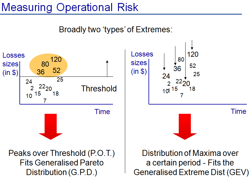
There are two main approaches under EVT:

The Block Maxima Approach or Block Method consists in observing and modeling the values of maximal losses. If we argue about the whole sample, we shall have only one maximum. To have a number of observations of maximum, it is necessary to cut the sample into Blocks and then to set maximum for every block. We obtain a number of maxima equal to the number of blocks. The theorem of Fisher Tippett supplies us the limit theorem for the maximum of normalized. This law is the law of the Generalized Extreme Value (GEV). The observed Maxima is then used to calibrate it.

Peaks Over Threshold (POT) Approach consists in considering the values beyond a threshold and either only the maximum. All the difficulty comes in choosing an appropriate threshold, which will allow to apply the Pickands theorem.

This theorem allows to model the excess by Generalized Pareto Distribution (GPD). This approach is used more usually than the approach of maxima because it allows to exploit more information supplied by the selected sample.

For a given distribution function G the generalized extreme value distribution (GEV), given by Gξ,μ,σ (x), describes the

limit distribution of suitably normalized maxima. Then G is necessarily in one of these three forms:

Fréchet	Weibull	Gumbel

These three distributions are the special case of the GEV (Generalized Extreme Value):

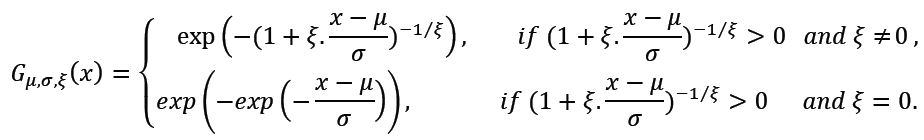
where μ, σ and ξ are the location, scale and shape parameters respectively.

• ξ  represents the index of extreme values. The more it will be higher in absolute value, the more the weight of extremes in the initial distribution will be important.
•  μ is the location parameter. It indicates approximately the heart of the distribution. 
• σ is the scale parameter. It shows the spread of extremes.

Fréchet	Weibull	Gumbel

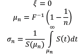Where S(X) = 1 – F(X) and x_F = sup{ x as F_X(x)< 1}.

 Copulas 

A copula is a function that joins multivariate distribution functions to the one-dimensional marginal distribution functions. Strictly speaking, a copula is a multivariate distribution whose one-dimensional margins are uniform on the interval [0, 1]. A n-dimensional copula (or n-copula) is a multivariate joint distribution defined on the n-dimensional unit cube [0, 1]ⁿ. In Operational Risk, Single Business Line (BL) has to be mapped to Multiple loss event types (ET) and there can be a possibility of multiple loss event types being linked to multiple BLs. Suppose two operational risks are thought to be positively dependent because the same risk drivers tend to increase both of these risks and the same risk drivers tend to decrease both of these risks. In that case the two loss distributions are aggregated to a total loss distribution via a copula with positive dependency. More generally, copulas can be chosen to reflect positive or negative dependencies that may

be different in the tails than they are in the center of the distributions.

In order to fairly assess the overall risk exposure, models have to take into account the correlation between individual risks when aggregating them. More importantly, models must capture the dependence between extreme events, thus reflecting the possibility of rare events cumulation. Copulas offer robust framework for correlation modeling. The Loss Distribution Approach (LDA) consists in modeling losses for individual risks and then aggregating them to calculate the overall loss distribution. The economic capital is computed as the Value-at-Risk at 99.9% confidence level for banks.

The distribution of a loss L_r for an individual risk r is seen as a mixture of two probability distributions. These two distributions represent two characteristics of a risk:

1. N_r represents the number of events caused by the risk r over a year. We say that N_r follows the frequency distribution.

2. X_r describes the severity of loss e.g. the amount of money lost each time an event occurs. We say that X_r follows the unit loss distribution.

Then the overall loss L_r for the individual risk r is given by:

We say that L_r follows the annual loss distribution for the individual risk r.

In Gaussian copula, dependence is determined by correlation and is therefore symmetric. In particular

the Gaussian copula underestimates the tail dependencies that are likely to arise with operational losses.

The Gumbel copula is useful for capturing asymmetric tail dependence, for example, where there is a greater dependence between large losses than there is between small losses. It can be parameterized in two ways. Many other copulas have been formulated, some of which have many parameters to capture more than one type of dependence. For example, a copula may have one parameter to model the dependency in the tails, and another to model dependency in the center of the distributions.

(3) Scorecard Approach (SCA)

The main disadvantage of actuarial methods is that they rely their estimates only on past data, thus reflecting a backward-looking perspective. Furthermore, for some business units, there are no loss data available at all. Regulators thus recommend to develop models that can take into account different data streams and not only internal loss data alone.

The scorecard approach is based on the Self Assessment, which is based on the experience and the opinions of a number of internal “experts” of the company, who usually correspond to a particular business unit. An internal procedure of control self assessment can be periodically done through questionnaires, submitted to expert risk managers, which gives information such as the quality of internal and external control system of the organisation on the basis of their own experience in a given period. In a more sophisticated version, experts can also assess the frequency and mean severity of the losses for such operational risks (usually in a qualitative way).

Representation of Self Assessment opinions

Self assessment opinions can be summarized and modeled so as to attain a ranking of the different risks, and a priority list of intervention in terms of improvement of the related controls.

In order to derive a summary measure of operational risk, perceived losses contained in the self-assessment questionnaire can be represented graphically (e.g. through a histogram representation) and lead to an empirical non parametrical distribution. Such a distribution can be employed to derive the 99,9% percentile Value at Risk.

Scorecard models are rather useful to prioritise interventions on the control system, so as to effectively reduce the impact of risks, ex ante and not a posteriori, as can be done by allocating capital (corresponding to the VaR).

Example of a methodology aimed at summarising concisely and effectively the results of a self-assessment questionnaire. Suppose that we are given 80 events at risk (this is the order of magnitude employed in typical banking operational risk management analysis). They can be traced to the four main causes of operational risk: People, Processes, Systems and External events. First of all a selected sample of banking professionals (both from the headquarters & the local branches) is obtained. The aims of the questionnaire project have been described in a group presentation. The nature and the structure of each risk question have been devised in a focus group discussion with the top manager of the bank.

The result of this preliminary analysis is that each of the selected professional is asked, for a total of about 80 risk events, his/her opinion on the: frequency, severity and effectiveness of the controls in place for each event.The number of possible frequency classes is equal to four: daily, weekly, monthly, yearly. The number of severity classes depend on the size of the capital of the bank, with an average of 6/7 classes, going from “an irrelevant loss” to “a catastrophic loss”.

Finally the number of possible classes of the controls are three: not effective, to be adjusted, effective.

Once interviews are collected, the aim is to assign a “rating” to each risk event, based on the distribution of the opinions on the frequency, controls and severity. Our proposal is to employ the median class as a location measure of each distribution, and the normalized Gini index as an indicator of the “consensus” on such location measure. This results in three rating measures for each event, expressed using the conventional risk letters: A for low risk, B for medium risk, C for higher risk and so on. While the median is used to assign a “single letter” measure, the Gini index is used to double or

triple the letter, depending on the value of the index. For example: if the median of the frequency distribution of a certain risk type (e.g. theft and robbery) is “yearly”, corresponding to the lowest risk category, a letter A is assigned. Then, if all interviewed agree on that evaluation (e.g. the Gini index is equal to zero), A is converted to AAA; if instead the Gini index corresponds to maximum heterogeneity A remains A. Intermediate cases will receive a double rating of AA. The same approach can be followed for the severity as well as for the controls, leading to a complete scorecard that can be used for intervention purposes. For visualisation purposes, colors are associated to letters, using a “traffic-light” convention: green corresponds to A; yellow to B; red to C and so on. Figure 1 presents the results from our scorecard model, for a collection of risk events belonging to People (Internal Frauds) and External Events (External frauds and losses at material activities)

Figure 1. Example of results from proposed scorecard model.

From Figure 1 it turns out that the event 1.2.6 should be given a priority 1 of intervention, as controls are not effective, and both frequency and severity are yellow. Other events at risk include 2.2.1 and 2.2.4 which have a high frequency and medium quality controls. We remark that the opinion on the severity is usually considered second in priority determination as it typically concerns a mean value which cannot be modified by the action of controls.

(4) Scenario Based Approach(sbAMA)

Historical data alone cannot be sufficiently indicative of an organisation’s operational risk. The complex underlying and dynamic causes of operational risk necessitate a progressive and proactive approach to risk management, drawing on all available information such as expert experience, internal and relevant external loss histories as well as key operational risk indicators and the quality of the control environment. sbAMA creates a forward-looking risk management framework that provides a direct link to business specific management actions and is responsive to changes in both the internal and external environment. The involvement of key stakeholders in the scenario generation and evaluation cycle creates risk awareness and supports the identification of management priorities.

Scenarios are potential future events. Their evaluation involves answering two fundamental questions: firstly, what is the potential frequency of a particular scenario occurring and secondly, what is its potential loss severity?  A representative set of scenarios are created that takes into account all relevant drivers of operational risk. The business of the bank depends on such risk factors (people, IT, process, controls) and is vulnerable if they fail, deteriorate or are of poor quality.

Risk factors can be categorized and thus give rise to Scenario Classes (SC) for example: IT breakdown. To derive scenarios from each of the scenario classes that are specific to a particular Business Line (BL), some form of organisational mapping (whether by product, process or business unit) is required. For each combination of SC and BL, scenarios will then be designed in the form of “what if” questions.

Application of sbAMA

The sbAMA is considered to be conceptually sound on the basis that information is only fed into a capital computation model if it is relevant to the operational risk profile of a Business Line and thus is needed to answer the “what-if” questions in the scenario assessment. Furthermore the overall sbAMA process must be supported by a sound and structured organisational OR framework and by an adequate IT infrastructure. The sbAMA comprises of six main steps, which are illustrated in the figure below.

Overview of the sbAMA

(5) Causal Modeling (Bayes Theorem)

Using a causal approach each operational loss depends on the outcome of other events (causes), each of which can also be dependent; for this reason it is suited for frequent events, with low severity. Although it is very difficult to specify the links between different events and “causal” factors, such as the internal/external audit process and other key risk indicators (on people, IT and processes), it is very useful for control and monitoring purposes. There can be positive correlation, negative correlation and zero correlation between and among different event types (ET) in different business lines (BL).

Parametric methods are based on parameters derived from a distribution. Historical data used for prediction. Regression analysis is performed, correlations are worked out and simulations are made for expected and unexpected losses.

In fact, the Bayesian statistical approach allows to integrate, via Bayes theorem, different sources of information coming from loss data collection, self assessment and external, industry loss data (data pooled) and opinion of risk managers, to give a unified knowledge which allows to manage OR (i.e., identification, assessment, monitoring and control/mitigation) and, at the same time, to determine minimum capital requirement better and more risk sensitive through Op VaR. This

allows to combine backward-looking historical data with forward-looking expectations and opinions and, at the same time, through Bayesian networks we can also consider the correlation between losses of different business lines and risk types and can evaluate the impact of “causal” factors. A Bayesian network is a set of nodes representing random variables and a set of arrows connecting these nodes in an acyclic manner.

Causal Modeling is used as an alternative to parametric methods. Causal models are based on Bayesian graphical models. Nodes represent variables and Links are conditional probabilities (implying causality). It has several advantages over parametric models.

A causal network consists of a set of variables and a set of directed links between variables. If there is a link from A to B we say A is a parent of B. Given a particular value for a variable, the probabilities are updated using a Bayesian approach. Several other variations are also available.(e.g. Markov network, Dependency Graph, etc.).

Bayes’ theorem relates the conditional and marginal probabilities of stochastic events A and B:

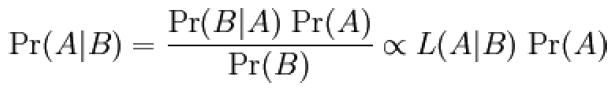
where L(A|B) is the likelihood of A given fixed B.

Each term in Bayes’ theorem has a conventional name:

– Pr(A) is the prior probability or marginal probability of A (does not take into account any information about B).

– Pr(A|B) is the conditional probability of A, given B (depends upon the specified value of B) and vice-versa.

– Pr(B) is the prior or marginal probability of B, and acts as a normalizing constant.

Paraphrasing: the posterior probability is proportional to the prior probability times the likelihood.

Obtain the likelihood function f(x|n).

– This step describes the process giving rise to the data x in terms of the unknown parameters n.

 Obtain the prior density f(n).

– The prior distribution expresses what is known about n prior to observing the data.

 Apply Bayes’ theorem to derive the posterior density f(n|x).

– This will now express what is known about n after observing the data.

 Derive appropriate inference statements from the posterior distribution.

– These will generally be designed to bring out the information expressed in the posterior distribution.

Risk Control & Self Assessment (RCSA)

Risk Control-Self Assessment is a risk management tool used by business managers to transparently assess risk and control strengths and weaknesses against a Control Framework. The “self” assessment refers to the involvement of management and staff in the assessment process. RCSA exercise helps in identifying potential weakness and inherent risks.

RCSA: Proactive Risk Identification & Management Tool

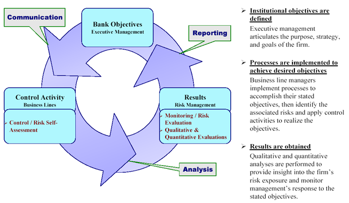
RCSA provides systematic means to identify Risk clusters (risk concentrations) and Control duplications/gaps or over-controls and to set up prevention & control measures and corrective action plans. 

Internal Audit in conjunction with Management Tool helps in building the synergy. Internal Audit Tool facilitates a risk-focused approach to Internal Audit while Management Tool, generally accepted to satisfy corporate governance & regulatory requirements. 

RCSA is proactive as opposed to Operational Loss Reporting. It allocates front line responsibility for ORM and place control directly with management – hence, corrective actions more effective & timely. It helps in creating a cultural change in the institution. 

RCSA AIM

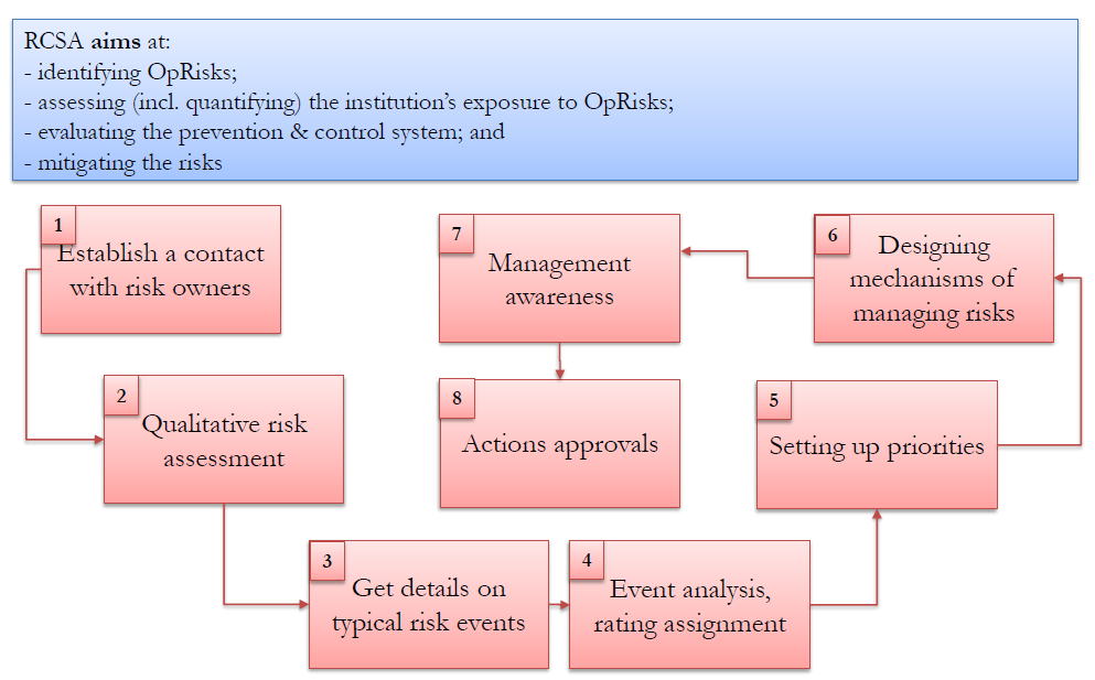
RCSA WORKFLOW

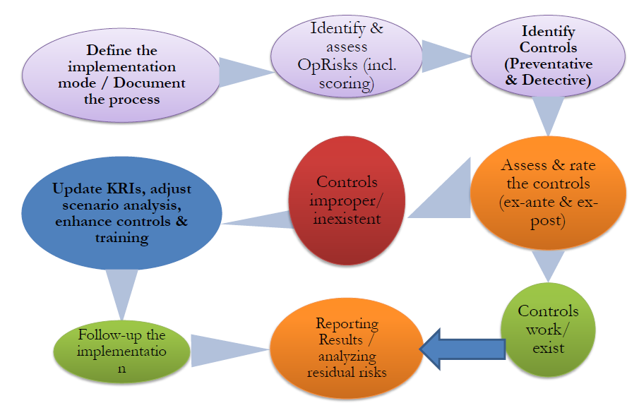
RCSA Methodologies

Workshop	Questionnaire	Hybrid
Evaluate business areas to address	Based on extensive /comprehensive questionnaire that identify risks	Comprehensive approach combining –top-down‖ (cascading from Executive Committee level, apportioned for each business line from a consolidated repository); and
Define Workshop objectives	Questionnaire shall: – determine standard controls, – benchmark standards, -evaluate the quality of actual performance	-bottom-up‖ (each business line identifies and routes-up. This is susceptible to duplication).
Engage professional impartial facilitator (record- keeper, devil‘s advocate, arbiter);	Choose between standard and non-standard (preferable) questions, ideally to be answered Y/N/NA	Initial workshop followed by a question-reply for future exercises + further workshops for any new activity or after a major OR event.
Select empowered staff to attend (including top management depends on the corporate culture)	Review the results to estimate residual OR profile, use them to determine remediating action
Max 3 modules (risk profiling; control assessment, action planning & ownership)
Data collection
Top management results sign-up required.

RCSA Toolkit- Sample Checklist

Sr No.	Questions	YES	NO	NA
1	Does the bank recruit staff with appropriate experience, skill levels and degree of expertise to undertake specialized business operations?
2	Do staff members actively take part in business operations in line with their position and responsibilities?
3	Does the bank recruit staff based on approved employment plan?
4	Does the bank perform background checks on all employees prior to hiring?
5	Does the Board have a clear policy on staff training?
6	Does the bank have a formal on-the-job training program for all major areas?
7	Does the bank use training programs according to qualifications and job description?
8	Is the training program proactive or reactive?
9	Does the bank revise training programs in accordance with changes in business scenarios and sophistication of risk management?
10	Is there any gender discrimination while recruiting people?
11	Is the recruitment process transparent in the bank?
12	Does the bank allow any form of favoritisms while recruiting?

• Used in initial survey 
• Yes/No answers 
• Needed for questionnaire 

Input required for Operational Risk Mapping from various stakeholders for RCSA.

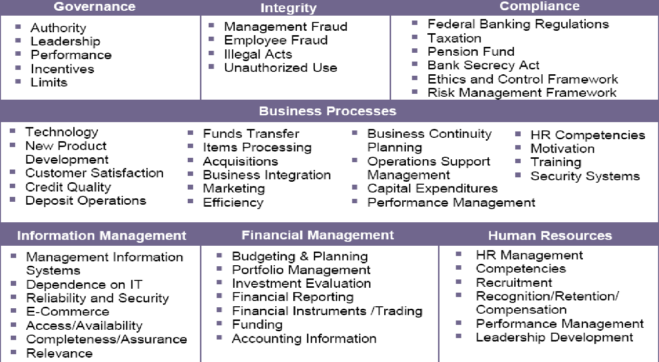
RCSA results are very useful and relevant for management decision making. It is an amalgamation of organizational goals, objectives and strategies with individual Business Line and line managers comprehension of risk management and effective risk control. 

RCSA exercise results in Management Reporting through Dashboards, Heat maps and Scorecards.

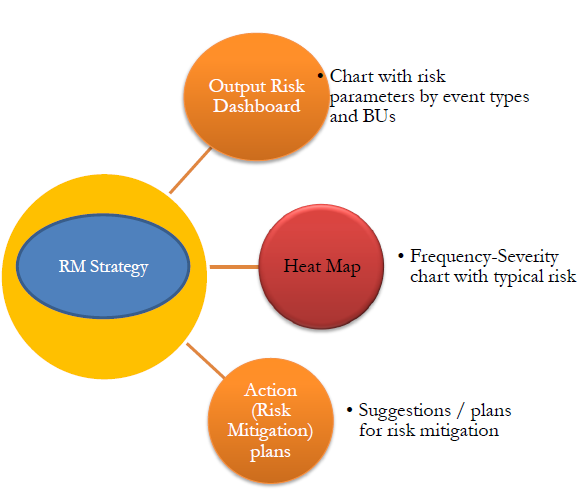
Sample Operational Risk FREQUENCY – SEVERITY RISK MAPPING

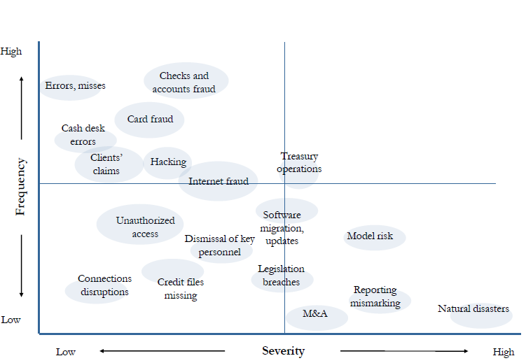
KEY RISK INDICATORS (KRI)

Risk and performance indicators are risk metrics and/or statistics that provide insight into a bank’s risk exposure. Risk indicators, often referred to as Key Risk Indicators (KRIs), are used to monitor the main drivers of exposure associated with key risks. Performance indicators, often referred to as Key Performance Indicators (KPIs), provide insight into the status of operational processes, which may in turn provide insight into operational weaknesses, failures, and potential loss. Risk and performance indicators are often paired with escalation triggers to warn when risk levels approach or exceed thresholds or limits and prompt mitigation plans. Analysis of operational risk drivers is still immature; finding satisfactory key risks indicators constitutes a challenge for many banks.

Davis (2007) states that KRIs sounds like a straightforward concept, measuring and reporting the items that may give cause for concern; however, there are many challenges associated with the concept, for example: 

 is the right thing being measured? 

 are the measures accurate? 

 are the definitions clear? 

 are truly key risk indicators identified? 

 how are the KRIs depicted? and 

 can the KRIs be used to determine the current risk exposures? 

According to Hoffman (2002), operational risks will not be effectively identified without first identifying the key risk indicators of operational risk. The main challenge in dealing with operational risk indicators is in identifying or constructing metrics that serve as predictors of operational risk. 

During the identification of the quantifying parameters of the risk indicators, the following aspects should be considered:

 the actual degree of severity, size of intensity that describes the observed extent of the presence of operational risk; 

 the frequency of risk existence and measuring their parameters – the frequency describes the number of times a risk of a given size occurs within a given period of time; 

 the context-dependency relation, which may differ in certain situations; and 

 the possible correlation and its sign with other indicators based on the common parameters among all indicators . 

 In addition, KRIs should have the following characteristics in order to be used as a tool to management operational risk: 

 the data must be available; 

 the data must be quantifiable in either percentage, value or volume; 

 a tolerance threshold must be determined by management and must only change according to changing circumstances, and 

 the KRIs must be monitored on a regular basis. 

The Institute of Operational risk (2010) furthermore states that indicators must be capable of being measured with a high level of certainty and on a repeated basis. Therefore, indicators should be numbers/counts, monetary value, percentages, ratios, time duration or a value of some pre-defined rating set. A very important aspect is that, when an indicator is identified, the measurement is agreed to by all stakeholders to ensure that everyone agrees what the value represents, how it is calculated, what is included or excluded and how variances in the values will be dealt with (Institute of Operational Risk 2010).

KRIs are the measures summarizing the frequency, severity and impact of OpRisk risk events or corporate actions occurred in the bank during a reporting period.

Risk dimensions	Indicators Type
Frequency	Number of risk events
Severity	Volume of risk events Average risk losses Maximum duration of disruptions
Impact	Total amount of risk losses Cost of mitigations

Sample Key Risk Indicators

Branch network • Number of complaints and claims to the Bank • Number of lost clients • Amount of compensation paid to the client • Volume of balances lost / opportunity cost	Loan / Client department • Average days of getting loan approval • Number of identified fraud cases • Client dissatisfaction evidenced by client surveys • Number of critical errors detected in credit files
Legal department • Number of legal actions against the Bank / third parties • Volume of legal actions against the Bank / third parties • Number of regulatory enquires / legislation breaches	Finance department • Volume of penalties, imposed by regulators • Total amount of suspicious transactions • Number of late completion or non-completed transactions
Human resources • Turnover of experienced staff • Number of temporary/short term staff • Number of employees, attended training courses • Number of employees, failed to pass mandatory evaluation	IT • Number of failures related to IT system and other equipment • Number of calls to help desk on IT system and other equipment • Average down-time of IT system and other equipment • Increase in transaction load on systems

Key Performance Indicators

KPIs are the measures that evaluate scale of banking activities. According to many empirical observations that is directly related to operational risk exposure.

Extension Risk • Gross Income • Total Assets • Book Value of Fixed Assets • Cost to Income	People Risk • Number of Employees • Staff Payroll • Income per Employee • Cost per Employee
Customer / Reputational Risk • Number of client accounts • Volume of client accounts • Average balance of single client account	Process Risk • Volume of transactions • Number of transactions • Average amount of single transaction

Key Control Indicators

KCIs are the measures that enables to monitor effectiveness of OpRisk management procedures established in the Bank, collected from business units, Risk management, Internal Audit reports, and Regulators.

Business Units • Number of breaches identified by the staff • Number of disciplinary actions taken • Percentage of loss mitigation	Risk management • Number of days before breaches are identified • Number of action plans introduced • Number of action plans failed to implement
Internal Audit • Number of breaches in processes identified by internal audit • Number of breaches eliminated	Regulators • Number of claims on the Bank in the area of OpRisk made by the regulator • Number of errors eliminated

SPECIFIC EVENT TYPES 

OpRisk event is an event leading to the actual outcome(s) of a business process to differ from the expected outcome(s), due to inadequate or failed processes, people and systems, or due to external facts or circumstances. 

 Single event 

 Repeated mistakes due to a process failure 

 Multiple impacts from a single cause 

 Fraud losses connected by a common plan of action 

 A technology outage which affects multiple business lines 

 Multiple errors made by a single individual over a period of time 

Linked event-a single event, which impacts more than one business line 

 the owner of the transaction 

 business process out of which the event arose 

 the business with the largest P&L impact 

 to multiple business lines based on P&L split 

SOURCE: Operational Risk Reporting Standards. ORX, Edition 2011

Observed range of practice in key elements of Advanced Measurement Approaches (AMA). BCBS, July 2009

Near-misses – operational risk events that did not lead to a loss, but had the potential to do so 

 IT disruptions outside working hours 

 Fault in transmitting erroneous mandatory reports 

 Cancelling doubled printed trading order 

 Grow cold when air condition system is out of operation 

 Operational risk gain events – operational risk events that generate a gain 

 Trading limit was not observed but position win 

 Product miss-selling that yield profit for the bank 

 Making mistake in setting FX rate that brought larger income 

SOURCE: Operational Risk – Supervisory Guidelines for the AMA. BCBS, June 2011

SPECIFIC LOSS TYPES

OpRisk loss – a negative and quantifiable impact on the P&L due to Operational Risk event.

 Single loss – a total amount of all Operational Risk losses pertained to a single loss event. 

 Grouped losses are Operational Risk losses with the same underlying cause that arise from single events within a Business Line and between Business Lines. For risk calculation and reporting purpose grouped losses have to be considered and recorded as a single ―root event.

 Root loss – the initial single event without which none of the grouped related losses would have occurred. 

Specific Loss Type Example

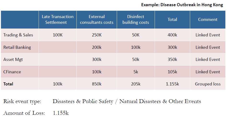
SOURCE: Operational Risk Reporting Standards. ORX, Edition 2011

Risk Report Sample

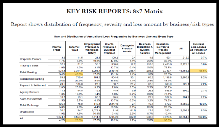
SOURCE: Results from the 2008 Loss Data Collection Exercise for Operational Risk. BCBS, July 2009

Operational Risk Mitigation

Business Continuity-Plans takes into account different types of likely or plausible scenarios to which the bank may be vulnerable. Continuity management incorporates: 

(1) Business impact analysis; 

(2) Recovery strategies, 

(3) testing, training and awareness, communication programs, 

(4) Crisis management programs 

Banks needs to identify critical business operations and key internal and external dependencies and appropriate resiliency levels and provide business continuity testing with key service providers. Disaster prevention aims to reduce threats of disaster before it occurs. Disaster recovery seeks to re-establish the critical functions after an interruption / disaster. The

4 core resources: people, location, IT and external services need to be protected.

Efficient management of disasters – arguably is more important to stakeholders than risk transfers.

Operational Risk Mitigation Tools

(1) Insurance: There are multiple benefits of Insurance. Basel II capital rules’ allows up to 20% off operational risk capital in recognition of insurance cover if the Bank is using the AMA method for determining the operational risk capital.. Insurance helps in removing Operational Risk to some extent from the balance sheet for a cost (premium) by providing a restrictive cover and (un)certain payment. Operational Risk is substituted with a counterparty/credit risk on an insurer. However, the Questions of Insurer‘s liquidity, loss adjustment, voidability, moral hazards, limits in insurance product range need to be assessed by the bank before entering into an agreement with the insurers. The 9/11 and Moscow terrorist attacks have made banks rethink insurability conditions and identify hidden exposures in insurance terms and conditions. Terrorism magnifies business interruption as a major Operational Risk.

Insurance does not protect reputation or ensure that business will continue. 

Challenges of using the insurance: 

-Selecting the right coverage 

-Incorporating the insurance policies into the capital allocation strategies; 

– Potential payment delays (critical for small credit institutions).

The following condition must be met for selecting the right insurance:

Must be related to actual risk exposure of bank to evidence need for mitigation,(e.g. catastrophe insurance in case of earthquake) 

• Insurance provider rated at least A 

• Insurance provider not to be related to banking group; unless re-insured via eligible re-insurer 

• Tenor of insurance 1 year for 100% recognition 

• If less than 1 year, apply haircuts, to reach 0% recognition if under 90 days 

• No exclusions or limitations as a result of regulatory action or events that took place before insolvency 

(2) Outsourcing Operations Risk

Operational Risk can be outsourced to some vendors/other organizations by banks. This helps in 

• Cost reduction 

• Higher process quality 

• Risk sharing/ transfer 

• Benefits from economies of scale; 

• Allowing better focus on core/new business; 

• Accessing new technology 

(3) Alternative Risk Transfers

Products	Product distinctive Features
Insurance-linked securities, including index securitization	Super catastrophes
Finite reinsurance Risk transfer + risk financing	– Multi-year; -particulars of each operational risk covered; -Possible sharing of financial results
CAT Bonds(catastrophe)	If no loss-event occurs, investors receive coupon If a defined catastrophic event takes place, investors lose interest, principal or both
Catastrophe swaps	Fixed payments exchanged for a series of floating that depend on occurrence of an insured event
Industry Loss Warranties	Resemble catastrophe swaps, structured as a reinsurance
Catastrophe options	Listed at Chicago Board of Trade

(4) Internal Measures

Some of the internal measures that act as mitigants to Operational Loss are Collateral Management, Netting Agreements in place, Limits Management and Audit Reports and control.

Standardised Approach, the new Basel 4 methodology for calculating Operational Risk Capital Requirement is based on the 3 components:

(1) Business Indicator (BI)- It is a financial-statement-based proxy for operational risk. The BI comprises three components: the interest, leases and dividend component (ILDC); the services component (SC), and the financial component (FC).

BI = ILDC + SC + FC

ILDC, SC and FC are defined in the formulae below, where a bar above a term indicates that it

is calculated as the average over three years: t, t-1 and t-2. The absolute value of net items (eg interest income – interest expense) should be calculated first year by year. Only after this year by year calculation should the average of the three years be calculated.

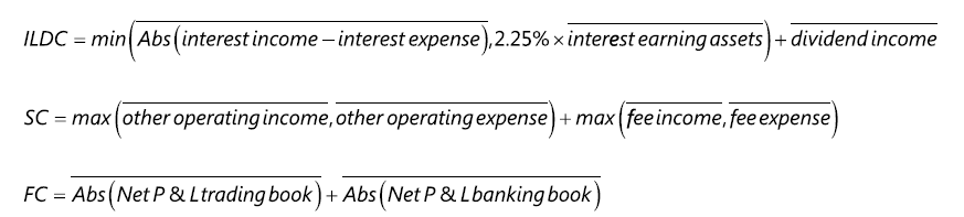
(2) Business Indicator Component (BIC) – It is calculated by multiplying the BI by a set of regulatory determined marginal coefficientsαi. Banks are classified into 3 different buckets as given in Table 1.

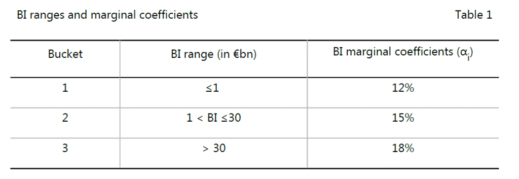
For example, given a BI = €35bn, the BIC = (1 x 12%) + (30-1) x 15% + (35-30) x 18% = €5.37bn.

(3) Internal Loss Multiplier (ILM) – It is a scaling factor that is based on a bank’s average historical losses and the BIC.

The calculation of average losses in the LC must be based on 10 years of high-quality annual loss data. When banks first become subject to calculation of the ILM, banks that do not have 10 years of high-quality loss data may use a minimum of five years of data to calculate the LC.3 Banks that do not have five years of high-quality loss data must calculate the capital requirement based solely on the BIC.

For risk management purposes, and to assist in supervisory validation and/or review, a supervisor may request a bank to map its historical internal loss data into the relevant Level 1 supervisory categories as defined in Table 2 and to provide this data to supervisors. The bank must document criteria for allocating losses to the specified event types:

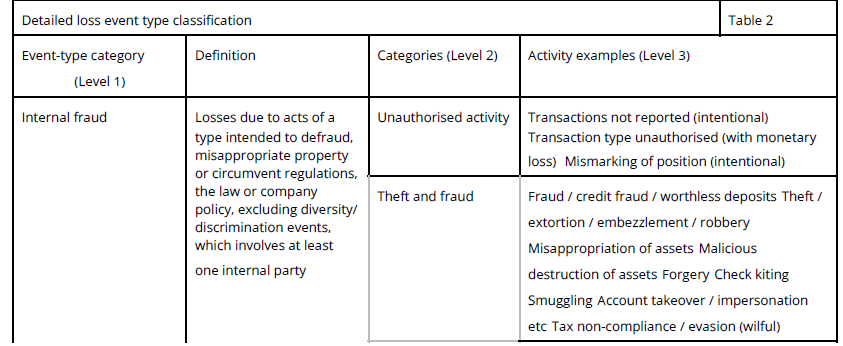
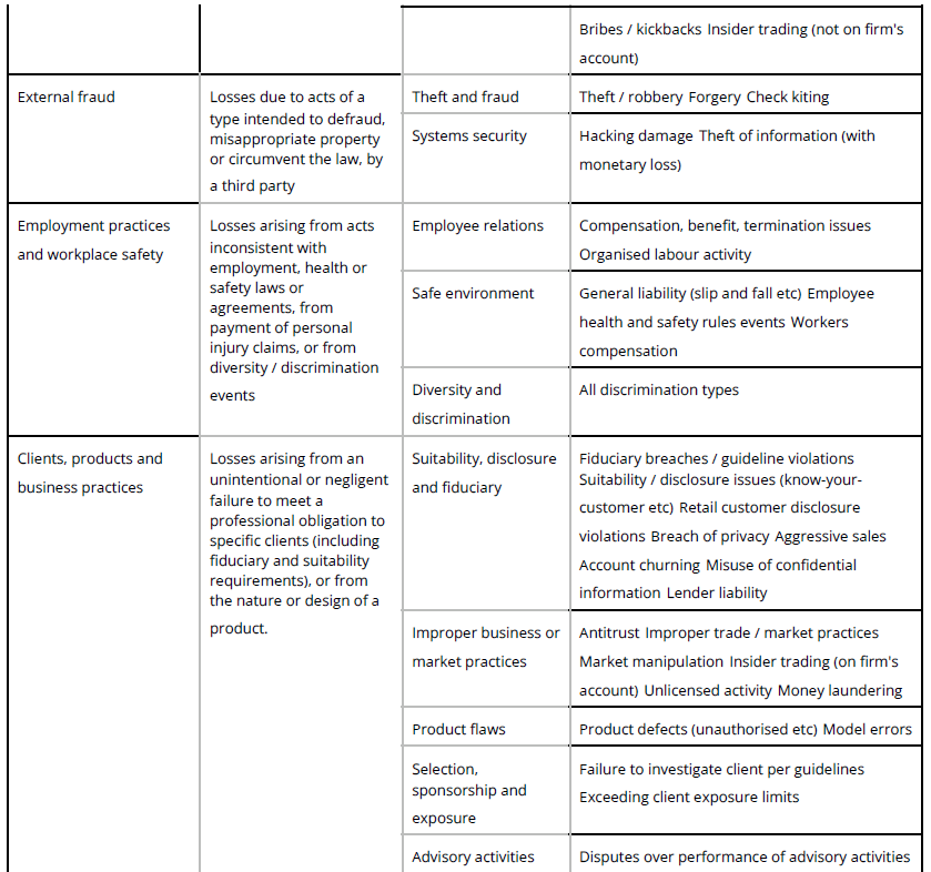
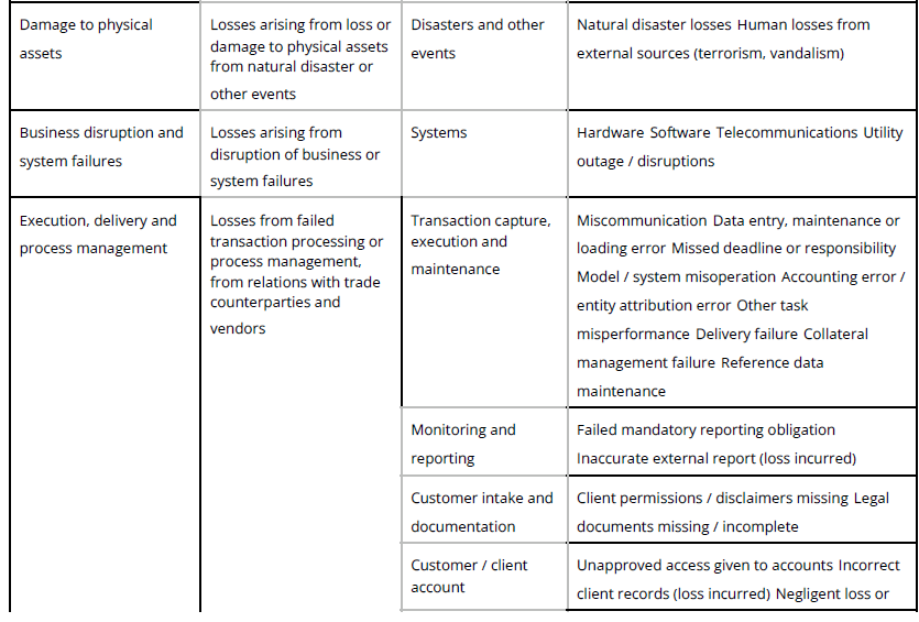
Operational Risk Capital (ORC) = BIC x ILM

RWA for Operational Risk = 12.5 x ORC.