Risk Overview: What is Market Risk?
Market risk can be defined as the risk of losses in on and off-balance sheet positions arising from adverse movements in market prices. From a regulatory perspective, market risk stems from all the positions included in banks’ trading book as well as from commodity and foreign exchange risk positions in the whole balance sheet. Capital for banks was based on a 10-day 99% VaR measure as allowed by the 1996 Basel I Amendment. The computation of VaR by most banks applied historical simulation. VaR is now being replaced by Expected Shortfall in Banks. Broadly speaking, market risk refers to changes in the value of financial instruments or contracts held by a firm due to unpredictable fluctuations in prices of traded assets and commodities as well as fluctuations in interest and exchange rates and other market indices. Market Risk includes Default risk, interest rate risk, credit spread risk, equity risk, foreign exchange risk and commodities risk for trading book instruments and Foreign exchange risk and commodities risk for banking book instruments.
Trading Book: The trading book includes all the assets that are marketable i.e they can be traded in the market. The trading book assets have the following characteristics. They are available for sale (AFS) or held for trading (HFT), normally not held until maturity and the positions are liquidated in the market after holding it for a period. Mark to market (MTM) system is followed and the difference between the market price and the book value is taken to P& L account. Trading book products are exposed to Market Risk including liquidation Risk, Credit Risk and Operational Risks.
Trading Book Instruments
The following instruments must be assigned to the trading book:
(a) short-term resale
(b) profiting from short-term price movements;
(c) locking in arbitrage profits;
(d) hedging risks that arise from instruments meeting criteria (a), (b) or (c) above.
(e) instrument in the correlation trading portfolio;
(f) instrument that is managed on a trading desk;
(g) instrument giving rise to a net short credit or equity position in the banking book;
(h) instruments resulting from underwriting commitments.
(i) instruments held as accounting trading assets or liabilities;
(j) instruments resulting from market-making activities;
(k) equity investment in a fund excluding banking book instruments (e);
(l) listed equities
(m) trading-related repo-style transaction;
(n) options including bifurcated embedded derivatives from instruments issued out of the banking book that relate to credit or equity risk.
Banking Book Instruments
The following instruments must be assigned to the banking book:
(a) unlisted equities.
(b) instrument designated for securitisation warehousing.
(c) real estate holdings.
(d) retail and SME credit.
(e) equity investments in a fund, including hedge funds, in which the bank cannot look through the fund daily or where the bank cannot obtain daily real prices for its equity investment.
(f) derivative instruments that have the above instrument types as underlying assets
(g) instruments held for the purpose of hedging a particular risk of a position in the types of instruments mentioned above.
VAR
VAR was first conceived by Dennis Weatherstone, the former Chairman of J P Morgan. He wanted to present a simple estimate of the maximum expected loss to BOD without showing complex statistics. Faced with this challenge, a team of researchers at J.P. Morgan came up with a solution called Value At Risk. The Report containing the VAR estimate was presented at 4.15 PM every day. This report became famous as the “415 Report”. They later made public their methodology through the Risk Metrics Technical Document series which subsequently became the market standard for VAR.
Value at Risk (VAR) : VAR measures the potential loss in value of a asset or portfolio over a defined period for a given confidence level. Thus, if the VAR on an asset is $100 MN at a one-week 95% confidence level, then there is a 5% chance that the value of the asset will drop more than $100 MN over any given week. VAR can be calculated for all types of assets. This means you can calculate VAR for interest rate risk, foreign exchange risk, credit risk and commodity price risk. Some firms add these individual VARs together to arrive at an overall VAR. You cannot do this with other risk measures.
VAR is calculated by three methods: Variance-Covariance Method, Historical Method & Monte Carlo Simulation Method. Regulatory VaR is computed at a 99% level of confidence over a one-day time horizon. The Daily VaR for MIS is computed at a 95% level of confidence over a one-day time horizon, which is a useful indicator of possible trading losses resulting from adverse daily market moves.
Factors impacting VAR Calculation
Four main factors influence the VAR calculation. They are given below:
Exposure: In general, larger the position, greater the risk. Therefore, large positions creates greater VAR.
Time Horizon: The longer the Bank intends to hold the position, the greater the VAR. So, normally, 10day VAR is greater than 1 day VAR. (But not by a factor of 10, only the square root of 10).
Confidence Level: If we want a VAR that is very unlikely to be exceeded, then we will need to apply more stringent parameters. All things remaining same, this will increase the VAR and make it less likely to be exceeded. 95% VAR will differ from 99% VAR.
Volatility: Volatility is measured by Standard Deviation. When we deal in risky assets that have a history of going up and down in price, or if market conditions alter to make the positions move up and down in price, the VAR will also tend to increase. There are two main measures of volatility: Historical and Implied Volatility. Historical volatility measures
how quickly historical return changes over time. The Historical volatility is the average variance from the mean and is estimated as: σ = √∑(Rt – Rm)2 / n-1 where
Rt = Daily Return and Rm = Average of Daily Returns, n = no of trading days in year = 252
Methods of calculating VAR
VAR is calculated by three methods: Variance-Covariance Method, Historical Method & Monte Carlo Simulation Method. Regulatory VaR is computed at a 99% Confidence Level while the Daily VaR for MIS is computed at 95% Confidence Level over a one-day time horizon, which is a useful indicator of possible trading losses resulting from adverse daily market moves.
Variance- Covariance Method – This is also known as Parametric Method/Analytic Method. There are essentially 2 analytic methods. VAR is simple to compute once the Means, Variance & Covariance are inputted. It is assumed that “Returns are normally distributed”. If the returns are not normally distributed, then the computed VAR will understate the true VAR. This model is good for portfolios where there is a linear relationship between risk and portfolio positions. It breaks down when the portfolio includes Options since the pay-offs on an Option are non-linear. We use Delta Gamma Model for such a portfolio.
Historical Simulation – This is the simplest way of estimating the VAR. The VAR for a portfolio is estimated by creating a hypothetical time series of returns on that portfolio. This model assumes that the distribution of past returns is a good & complete representation of expected future returns. In a market where risks are volatile and structural shifts occur at regular intervals, this assumption is difficult to sustain. Moreover, in historical simulation all data points are equally weighted, so volatility is ignored. This model cannot be applied to new products as they don’t have any historical data.
Monte Carlo Simulation – This method allows for the most flexibility in terms of choosing distribution for returns and bringing in subjective judgments and external data. Monte Carlo simulations can be used to assess the VAR for any type of portfolio and are flexible enough to cover Options and Options like securities.
Benefits & Limitations of VAR
Benefits of VAR
1.VAR is used in the performance evaluation of Individual Trader or Trading Desk by linking the return to VAR.
2. VAR plays a crucial role in internal capital allocation set aside to cover the market risk.
3. VAR is used to set Trader & Desk, Product Limits.
4. VAR
Limitations of VAR
VAR is just one number and in that sense becomes a lot easier to calculate, understand and monitor it and Banks use it across the globe.
VAR is not a maximum loss figure. From time-to-time, we may find that the actual amount of money lost exceeds the VAR.
VAR takes into account only Market risk and does not consider Political risk, Liquidity Risk , Operational Risk and Regulatory Risk.
VAR cannot capture adequately credit risk and unable to capture market liquidity risk.
VAR also does not capture effectively the tail risk and basis risk.
VAR can be computed over a quarter or a year but it is usually computed over a Day/Week. So in real world, it is computed for short time periods. Large and potentially catastrophic events that are extremely unlikely in a Normal distribution but seem to occur at regular intervals in the real world, are not captured by VAR.
FRTB
BCBS issued the revised minimum capital requirements for market risk on January 14, 2016. The revised framework is the culmination of the three Fundamental Review of the Trading Book (FRTB) during the consultative phase. The revised market risk capital framework is aimed at plucking the outstanding structural shortcomings observed during the global crisis within “Basel 2.5” by addressing the undercapitalisation of the trading book. The new rules came into effect in 2019.
Key Objectives of FRTB
Global financial crisis of 2007-08 highlighted significant weaknesses in trading activities of banks. Consequently, BCBS undertook the Fundamental review of the trading book to improve the overall design and coherence of the capital standard for market risk. Some of the key objectives of the new market risk framework are:
- Discouraging window-dressing by banks as far as possible.
- Discouraging banks from taking excessive intraday exposures.
- Plucking the loopholes for capital arbitrage between trading & banking book.
- Stopping the switching of instruments between trading & banking book as far as possible.
- To create a clear demarcation between Banking Book & Trading Book for computing the regulatory capital requirement for market risk.
- To ensure that the bank takes immediate measures to rectify the situation if it fails to meet the capital requirements at any time.
- To captures the credit risk inherent in trading exposures.
- To capture “tail risks” so that large unexpected losses could be identified and avoided.
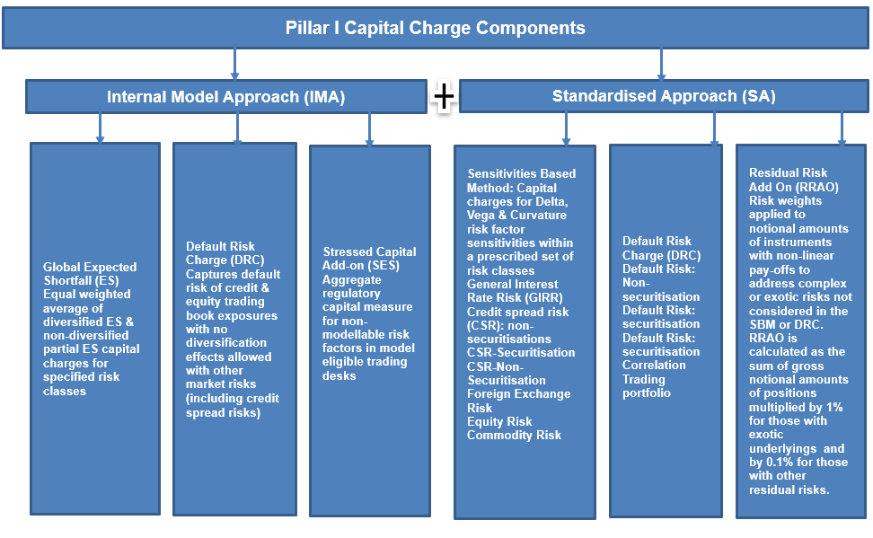
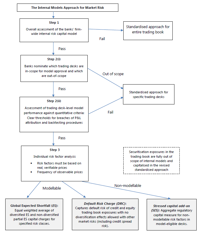
Banks can either use their own Internal Models Approach or Standardised Approach to calculate capital under FRTB. For the Trading Desk to qualify for the internal model approach, they must pass Two tests: 1. Profit & Loss Attribution Test 2. Backtesting.
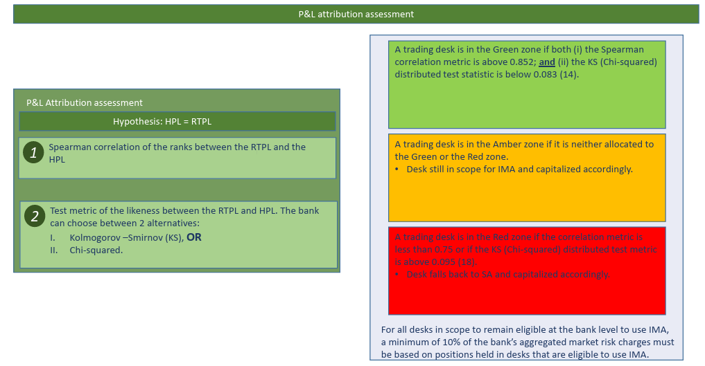
The P & L Attribution Test compares the profit and loss generated by a Bank’s front office pricing system with the figures generated in the back office for risk measures. Backtesting compares the P & L values with the VAR figures. In both the tests, if a Bank’s own estimates are found to deviate excessively from realised P & L for a given Desk over a 12month period, the Desk risks losing IMA approval and being forced to use the Standardised Approach. Banks using the IMA must calculate the Expected Shortfall (ES) measure to calculate capital as well as applying capital add-ons for risk factors that lack sufficient data for modelling. These are known as non-modellable risk factors.
ES replaces VaR & Stressed VAR. ES captures the tail risks that are not accounted for in the existing VaR measures. ES is supposed to capture the extreme losses that are normally not captured by VaR or SVaR but seem to occur quite frequently now a days.DRC model replaces the IRC model. Securitisation is completely out of scope of IMA and is to be calculated under SA method.
FRTB- Internal Model Approach Vs Standardised Approach- Market Risk
IMA Overview
Trading Desk Eligibility: Nomination for IMA
Banks must nominate which trading desks are in-scope for model approval and which trading desks are out-of-scope. Banks must specify in writing the basis for the nomination . Banks must not nominate desks to be out-of-scope due to standardised approach capital charges being less than the modelled requirements. Desks that are out-of-scope will be capitalised according to the standardised approach on a portfolio basis.
Trading Desk Eligibility to use IMA
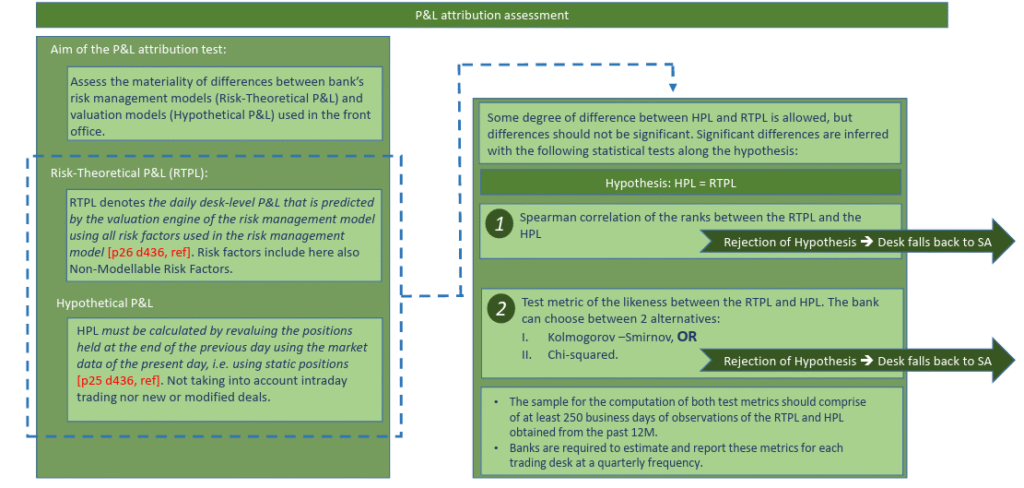
Trading Desk Eligibility to use IMA-P & L Attribution Assessment & Back Testing
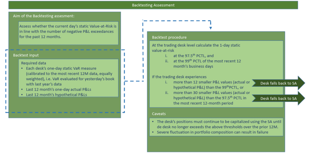
Back Testing Under FRTB
Back Testing Results have been divided into 3 Categories. Deals with Model’s accuracy level.
Green Zone: The Back Testing Results are supposed to be in green zone if the number of exceptions produced is between 0 and 4 in a sample of 250 observations. Number of exceptions is multiplied by a Multiplier to generate the Cumulative Probability. As the number of exceptions increases, the Multiplier is also increased.
Yellow Zone: The Back Testing Results are supposed to be in yellow zone if the number of exceptions produced is between 5 and 9 in a sample of 250 observations. Number of exceptions is multiplied by a Multiplier to generate the Cumulative Probability. As the number of exceptions increases, the Multiplier is also increased. The supervisor will impose a higher capital requirement for any outcomes that place the bank in the yellow zone.
Red Zone: The Back Testing Results are supposed to be in red zone if the number of exceptions produced is 10 or more in a sample of 250 observations. Number of exceptions is multiplied by a Multiplier to generate the Cumulative Probability. As the number of exceptions increases, the Multiplier is also increased. Red Zone implies that the models are inaccurate. Supervisory intervention increases to improve the model accuracy.
| Backtesting Zone | Number of exceptions | Backtesting dependent Multiplier | Cumulative Probability |
| Green Zone | 0 | 1.50 | 8.11% |
| 1 | 1.50 | 28.58% | |
| 2 | 1.50 | 54.32% | |
| 3 | 1.50 | 75.81% | |
| 4 | 1.50 | 89.22% | |
| Yellow Zone | 5 | 1.70 | 95.88% |
| 6 | 1.76 | 98.63% | |
| 7 | 1.83 | 99.60% | |
| 8 | 1.88 | 99.89% | |
| 9 | 1.92 | 99.97% | |
| Red Zone | 10 or more | 2.00 | 99.99% |
The uniform 10-day liquidity horizon as originally proposed in Basel regulations is inappropriate. This is because it is nearly impossible for banks to exit all risk positions within a 10-day period due to market illiquidity. As such, five different liquidity horizons have been proposed under FRTB: 10 days, 20 days, 40 days, 60 days, and 120 days. For example, the calculation of regulatory capital for a 120-day horizon (essentially 6 months’ worth of trading days) is intended to shield a bank from significant risks while waiting for six months to recover from underlying price volatility. The new proposals specify a liquidity horizon for each major risk factor. The following is a list of risk factors and the corresponding liquidity horizons:
Risk Factor Liquidity Horizons
| Risk Factor Horizon | (days) |
| Interest rate (dependent on currency) | 10-60 |
| Interest rate volatility | 60 |
| Credit spread: sovereign, investment grade | 20 |
| Credit spread: sovereign, non-investment grade | 40 |
| Credit spread: corporate, investment grade | 40 |
| Credit spread: corporate, non-investment grade | 60 |
| Credit spread: other | 120 |
| Credit spread: volatility | 120 |
| Equity price: large cap | 10 |
| Equity price: small cap | 20 |
| Equity price: large cap volatility | 20 |
| Equity price: small cap volatility | 60 |
| Equity price: other | 60 |
| Foreign Exchange rate (dependent on currency) | 10-40 |
| Foreign exchange volatility | 40 |
| Energy price | 20 |
| Precious metal price | 20 |
| Other commodities price | 60 |
| Energy price volatility | 60 |
| Precious metal volatility | 60 |
| Other commodities price volatility | 120 |
| Commodity (other) | 120 |
Calculating the Expected Shortfall Using the Internal Models Approach
In line with the proposals under FRTB, the internal models’ approach (IMA) requires banks to estimate stressed ES with a 97.5% confidence. Once risk factors have been allocated liquidity horizons as indicated in the table above, they are put into the following 5 categories:
- Category 1: Risk factors with 10-day horizons.
- Category 2: Risk factors with 20-day horizons.
- Category 3: Risk factors with 40-day horizons.
- Category 4: Risk factors with 60-day horizons.
- Category 5: Risk factors with 120-day horizons.
The use of these five categories is informed by the fact that risk factor shocks might not be correlated across liquidity horizons. Under the IMA, the expected shortfall is measured over a base horizon of 10 days. The expected shortfall is measured through five successive shocks to the categories in a nested pairing scheme. First, banks calculate ES when 10-day changes are made to all risk factors, with the resulting ES denoted ES1. Next, they are required to calculate ES when 10-day shocks are made to all risk factors in categories 2 and above but holding category 1 constant (The resulting value is denoted ES2). The process continues with ES calculation when 10-day changes are made to all risk factors in categories 3 and above but holding categories 1 and 2 constant (the resulting value is denoted ES3). They are then required to calculate ES when 10-day changes are made to all risk factors in categories 4 and 5 with risk factors in categories 1,2, and 3 being kept constant (the resulting value is denoted ES4). Finally, 10-day changes are made to risk factors in category 5 (the resulting value is denoted ES5).
Standardised Approach 7 Risk Classes

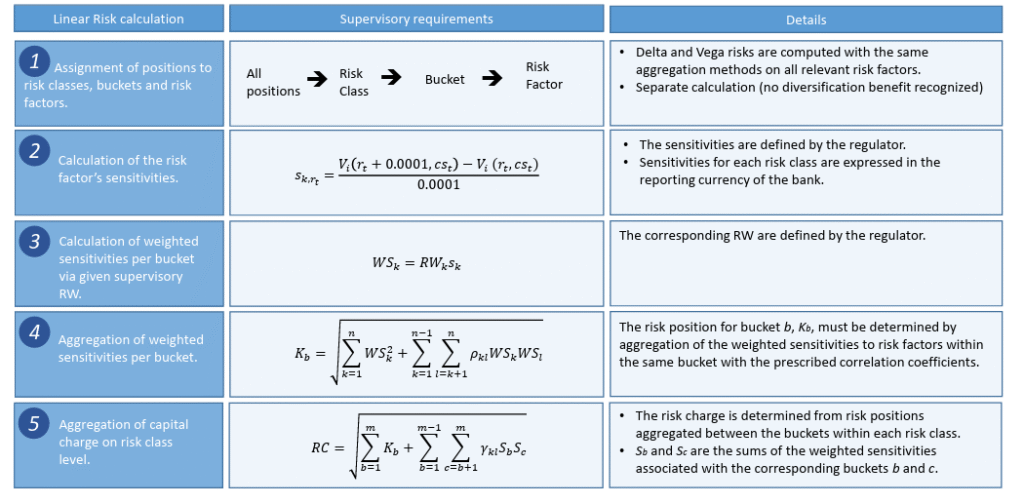
Standardised Approach- Delta and Vega Risk
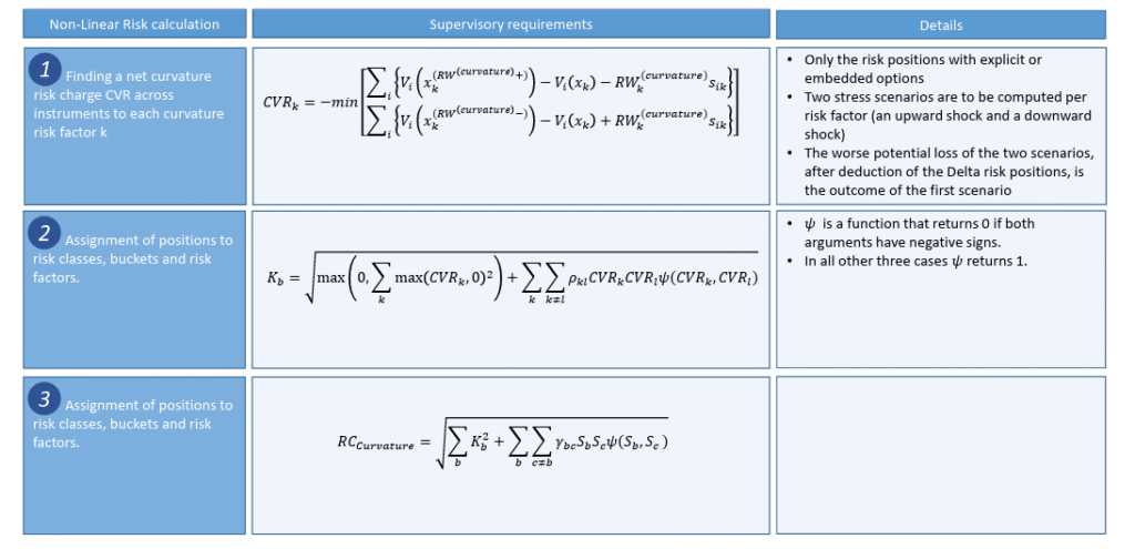
Standardised Approach- Curvature Risk
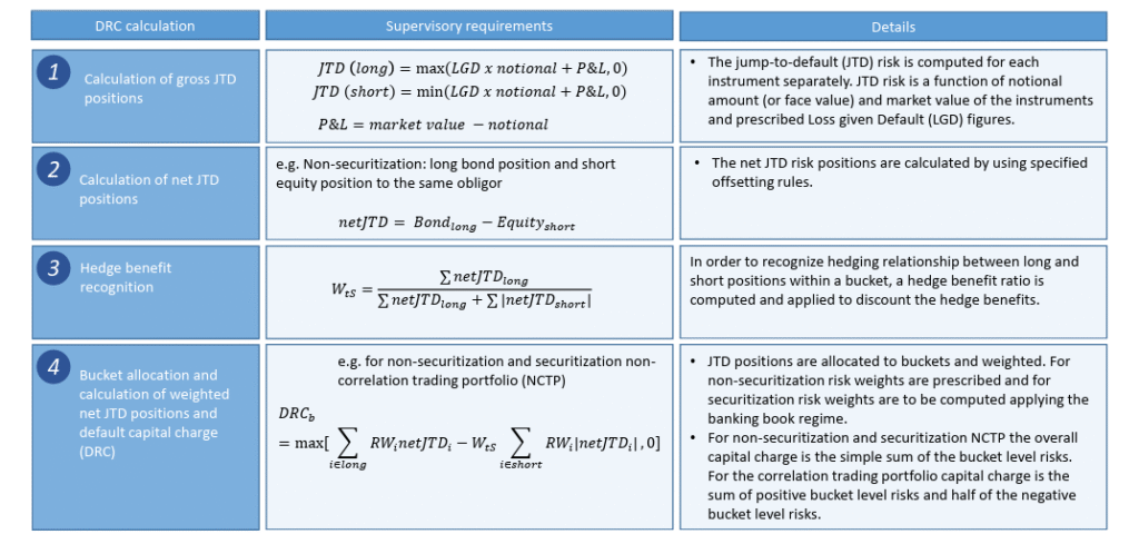
Standardised Approach-DRC Calculation
Components of Market Risk
Market risk comprises of the following risks:
Equity Price Risk :would include risk of potential losses due to fluctuations in prices of stocks and levels of Indexes. Positions involving long/short on stocks, stock futures, index futures and various options on either stocks or indexes would have equity price risks.
Interest Rate Risk : Banks being in the business of borrowing and lending money are most vulnerable to interest rate risks. Apart from loans and deposits, bonds and government security prices also vary with interest rates. Banks having portfolio of instruments like loans, deposits, bonds, Interest rate swaps, bond options, interest rate options etc. are exposed to this kind of risk.
Commodity Price Risk : would include risk of potential losses due to fluctuations in prices of various commodities. Positions involving long/short on commodities futures, commodity index futures and various options on commodities as well as owning commodities physically exposes the financial institutions to commodity price risks.
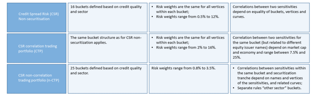
Credit Spread Risk : Banksthat takes positions in credit instruments, such as bonds & credit derivatives, is exposed to the risks of changes in the credit spreads of the underlying issuers. Credit spread is premium above government or risk-free risk, required by the market for taking on credit exposures. Credit spread risk is the risk that a company’s credit spread will change, causing the mark-to-market value of the instrument to change.
FX Risk :Risk arising from exposure towards different foreign currencies across various products is classified as FX (Foreign Exchange Risk).
Cross Asset Price Risk :Risks due to change in prices of not only one asset or even assets belonging to a single asset class. These are generally observed on structured trades which are done on a basket of assets and where the weights of particular assets in a basket are dependant on their relative prices and price returns.
Vega Risk : It is defined as the rate of change of the value of a portfolio with respect to the volatility of an underlying asset. Vega can be an important Greek to monitor for an option trader, especially in volatile markets, since the value of some option strategies can be particularly sensitive to changes in volatility.
Skew Risk: When implied volatility is plotted against strike price, the resulting graph is typically downward sloping for equity markets, or valley-shaped for currency markets. For markets where the graph is downward sloping, such as for equity options, the term “volatility skew” is often used. For other markets, such as FX options or equity index options, where the typical graph turns up at either end, the term “volatility smile” is used. Skewness in risk denotes that observations are not spread symmetrically around an average value. Skew risk is widely observed for volatility in options markets.
Volatility of Vol Risk :Advanced option pricing models do not take a constant volatility as a input instead the take stochastic volatility. What this means is that volatility itself is considered to be variable and this gives rise to another type of risk which is due to volatility in calculating volatility of an asset.
Correlation Risk: This comes from the fact that the prices of assets tend to move in tandem, even if they do not move in tandem they are at least not completely independent and uncorrelated. This type of risk is highlighted for portfolios having basket trades.
Market Liquidity Risk :It is the risk that an institution is unable to easily liquidate or offset a particular position without incurring lossess due to inadequate market depth or market disruptions. This can happen in a highly volatile market or due to some adverse development related to a specific company.
Basis Risk : arises when a hedge for particular financial instrument is not perfect i.e. the price changes in entirely opposite directions from each other. Example would be a spot position being hedged by a future, for this situation basis risk could arise because of the difference between the asset whose price is to be hedged and the asset underlying the derivative or because of a mismatch between the expiration date of the futures and the actual selling date of the asset.
Inflation Risk : The value of assets or income will decrease as inflation increases. Inflation Risk will shrink the purchasing power of a currency.
Credit Valuation Adjustment Risk: Another source of risk in derivatives position across asset classes is counterparty credit risk. Counterparty Credit Risk arises from the probability of the counterparties not honouring their obligation in particular trade when due. CVA is the process through which counterparty credit risk is valued, priced and hedged. In other words, CVA is the Market Price of Counterparty Credit risk.
Model Risk : It is the error in risk measurement or valuation that arises from the fact that modeling assumptions are imprecise and/or become invalid over time.
IRC: The Incremental Risk Charge represents an estimate of the default and migration risks of unsecuritised credit products over a one-year time horizon at 99.9 % confidence level, taking into account the liquidity horizons of individual positions or sets of positions. Includes flow products like bonds, CDS, listed equities.
CRM: Comprehensive Risk Measure is an estimate of risk in the correlation trading portfolio, taking into account credit spread, correlation, basis, recovery and default risks. The CRM is calculated at 99.9% confidence level over a one-year time horizon, applying the constant level of risk assumption.
Market Risk Management – Impact of Losses
BARINGS PLC – lost $ 1.3 Bn in 1995 – unauthorized trading by Nick Leighson.
SG – € 4.9 Bn Net in Jan 2008 – unauthorized trades, false hedges, risk measured on net basis, password management, knowledge of controls, weak controls; ―culture of tolerance‖, ignoring warning signs, incentive structure of traders etc.
London Whale – In September 2012, JPMorgan Chase trader Bruno Iksil (nicknamed the London Whale) gambled big on an obscure corner of the credit market—and lost in spectacular fashion. The London Whale not only incurred $6.2 billion in trading losses but allegedly also mismarked some of the losses to cover up their magnitude. His supervisor, Javier Martin-Artajo, was sued by the bank for assisting in the cover-up, JP Morgan Chase agreed to pay four regulators $920m(£572m) relating to a $6.2bn loss incurred as a result of the “London Whale” trades. The settlement is the third biggest banking fine by US regulators, and the second largest by UK regulators.
UBS – In early September 2011, the Swiss bank UBS announced that it had lost USD $ 2.3 billion dollars, as a result of unauthorized trading performed by Kweku Adoboli, a director of the bank’s Global Synthetic Equities Trading team in London. Britain’s financial regulator fined UBS $47.5 million for failing to prevent a $2.3 billion loss caused by this activity. trader.
The Greeks …Risk Metrics
The Greeks are vital tools in risk management. Each Greek measures the sensitivity of the market value of an Asset or Portfolio to a small change in a given underlying parameter, so that component risks may be treated in isolation and the portfolio can be rebalanced accordingly to achieve a desired exposure and return.
They are called the Greeks because four out of the five are named after letters of the Greek alphabet. Vega is the exception. For reasons unknown, it is named after the brightest star in the constellation Lyra. At times, Vega has been called Kappa, but the name Vega is now well established.
Four of the five are Risk metrics. Theta is not because the passage of time is certain – it entails no risk. Theta is akin to the accrual of interest on a bond.
Delta (Δ): The delta of an option is the rate of change in the value of the option with respect to change in the price of the underlying assets of the option. It is the first order sensitivity.
Rho (ρ): Rho of an option is the rate of change in the value of an option with respect to change in the level of interest rates.
Theta (θ): The theta of an option is the rate of change in the value of the option with respect to passage of time, with all else remaining the same. It is also called the “time decay” of the option.
Vega (ν): The Vega of an option is the rate of change in the value of the option with respect to volatility of the underlying assets of the option.
Gamma (Г): The gamma of an option is the rate of change of the option’s delta with respect to the change in the price of the underlying assets of the option.
Basel III impact on Market Risk: IRC & CRM
Basel III introduced Incremental Risk Charge and Comprehensive Risk Measure on the Trading Book of the Bank.
Incremental Risk Charge (IRC) is a regulatory capital charge for default and migration risk arising from positions in the Trading Book of the Bank. Covers corporate bonds, CDS, equity, correlation products but Not securitizations. The IRC is an estimate of default and migration risk of unsecuritized credit products in the trading book. The IRC model also captures recovery risk and assumes that average recoveries are lower when default rates are higher. The IRC is calculated at 1 year VAR at 99.9% confidence level . A constant level of risk assumption is imposed and ensures that all positions in the IRC portfolio are evaluated over the full one-year time horizon.
The Comprehensive Risk Measure (CRM) is an estimate of risk in the correlation trading portfolio, taking into account credit spread, correlation, basis, recovery and default risks. The CRM is calculated at a 1year VAR at 99.9% confidence level, applying the constant level of risk assumption. All positions in the CRM portfolio are given a liquidity horizon of 6 months. Comprehensive Risk Measure (CRM) includes specific risk and default and migration risk but also other price risks where relevant such as cumulative risk arising from multiple defaults , credit spread risk, volatility of implied correlations, basis risk, recovery rate volatility, and the risk of hedge slippage and the potential costs of rebalancing such hedges.
CVA
Previously, valuation of counterparty credit risk has largely been ignored due to relatively smaller size of the derivative exposures and the high credit rating of the counterparties which were generally AAA or AA rated financial institutions.
As the size of the derivative exposure increases and the credit quality of the counterparties deteriorated over the time, the valuation of counterparty credit risk can no longer be assumed to be negligible and must be appropriately priced and charged for. Credit Valuation Adjustment or CVA is the process through which counterparty credit risk is valued, priced and hedged.
How is it calculated?
The methodology to calculate both Asset CVA & Liability CVA is similar. In the formula below, we do not differentiate between asset/liability CVA.CVA is the expected value of credit losses over the lifetime of the trade. i.e.
CVA at each time bucket = PV (EAD * (1 – Recovery Rate) * Probability of Default) where
EAD = Exposure at Default at each time bucket. This is predicted by EPE/ENE profiles where
EPE/ENE = Expected Positive and Negative Exposures of the portfolio. These are generated using the market implied volatilities of market risk factors.
Probability of Default = Derived through market CDS spreads
Bilateral CVA is the sum of asset and liability CVA at each tenor bucket over the life of the trade.