Risk Overview: What is Risk?

• Risk is present everywhere in every form in all our activities. Risk can be defined as the possibility or threat of damage, injury, liability, loss or any other negative occurrence that is caused by external or internal factors and likely to impact adversely. Risk can never be eliminated totally but only mitigated to a large extent through preemptive action.
• Here, we will discuss only Credit Risk in this section. Credit Risk arises due to uncertainty in a counterparty’s ability to meet its obligation. Counterparties can be:
• Other Financial Institutions
• Corporates
• Sovereign Governments
• Individuals

Meaning & Definition of Credit Risk

Credit risk exists whenever a product or service is availed with a promise to settle payment in future, as agreed upon.

Credit Risk can be defined as “the probability of the loss (due to non-recovery) emanating from the credit extended, as a result of non-fulfillment of contractual obligations arising from unwillingness or inability of the counter-party or for any other reason”. If the probability of loss is high, the credit risk involved is also high, and vice versa.

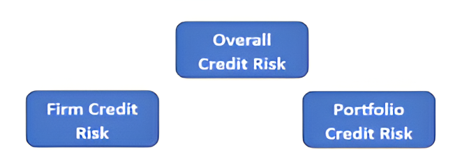
A single obligor exposure is generally known as Firm Credit risk while the credit exposure to group of similar obligors is called portfolio credit risk.

Causes of Credit Risk

Credit risk is subtle and hidden and has to be unearthed carefully, especially in view of the fact that the returns for credit risk are much lower than for other kinds of investments.

Both firm credit risk and portfolio credit risk are triggered by systematic and unsystematic risks.

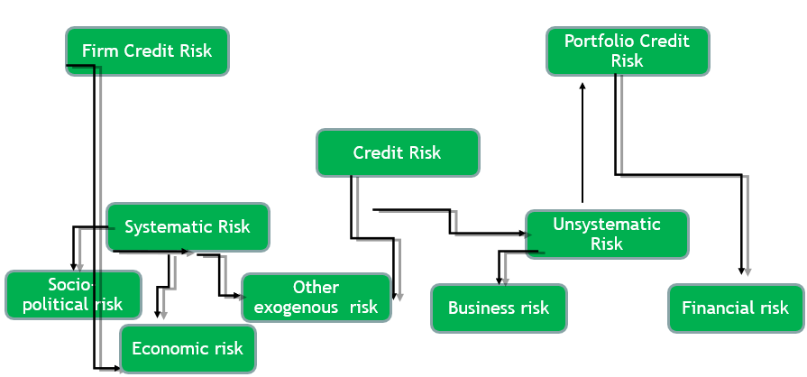
External forces that affect all businesses and households in the country or economic system are called systematic risks and are considered as uncontrollable risks. For instance, if the economy is witnessing a sharp economic crisis/recession, bankruptcies will increase triggering credit losses, while stock market will decline due to lower corporate profits while unemployment rises among others. Thus, systematic risks impact all in the playground.

The second type of credit risks, the unsystematic risks/unique risks that do not affect the entire economy or all business enterprises/households. Such risks are largely industry specific or company specific and unique to them. Thus, unsystematic risks can be eliminated or mitigated to a large extent.

Impact of Credit Losses

• The Bank suffers huge financial loss because of such activities.
• There is sudden loss of job and closure of business line.
• Sudden change in the business model of the bank.
• Regulatory and public pressure increase.
• Since, many a times, Banks/FIs are bailed out by Govt. and public money is used for bailing out, there is great political fall out. Economy suffers because of political fall out.
• Because of one blunder from one Bank, the whole Banking Industry suffers.
• The Market in general become bearish about that bank and the banking industry.
• There is great reputational loss for the bank and acts as a demoralizer.
• There is great loss of confidence in banking industry and both retail & Corporate Clients won’t like to do business in such an environment.
• If the loss keeps on mounting and spreads across the global banks, like it happened in US Sub-prime Case, it engulfs the whole world and results in a prolonged Depression. The crime increases in Society. The individual and the society changes permanently.
• UBS – credit write-downs related to sub-prime exposure of $ 37.7 Bn. S&P downgraded rating one notch to AA-. Tier 1 ratio fell to 7% without capital increase and rights issue.
• Citigroup – Write-downs on the value of loans, MBS and CDOs due to the subprime mortgage crisis of $ 39.1 Bn.
• For regulatory and reporting purposes, Banks measure the credit risk in terms of the money the bank expects to lose in the case of a counterparty defaults.
• Credit Risk is important because of:
• Subprime MBS Crisis
• Lehman Brothers collapse
• European sovereign debt crisis

Banking & Trading Book

Banking Book: The banking book includes all advances, deposits and borrowings which usually arise from commercial and retail banking operations. All assets and liabilities in banking book have following characteristics.

• They are normally held till maturity (HTM).
• Accrual system of accounting is applied.

Banking books products are exposed to Liquidity Risks, Interest Rate Risk, Credit Risk and Operational Risks. Since it is not open to market price, it is not exposed to Market Risk.

Trading Book: The trading book includes all the assets that are marketable i.e they can be traded in the market. The trading book assets have the following characteristics.

• They are available for sale (AFS) or held for trading (HFT) , normally not held until maturity and the positions are liquidated in the market after holding it for a period.
• Mark to market (MTM) system is followed and the difference between the market price and the book value is taken to P& L account.
• Trading book products are exposed to Market Risk including liquidation Risk, Credit Risk and Operational Risks.

Off Balance Sheet Exposures in Banks

Off Balance sheet Exposures: Off Balance Sheet Exposure are theAssets and Liabilities of the Bank but they do not appear on the Balance sheet. Off Balance sheet exposures are contingent in nature. Where banks issue Guarantees, committed or back up credit lines, Letters of Credit, Standby Letter of Credit (SBLC), Revolving Underwriting Facilities (RUF) , banks face payment obligation contingent upon some event such as failure to meet payment obligation by the principal parties. Additionally, swaps, futures, forwards, and option contracts are derivative instruments whose notional values are carried off-balance sheet, but whose fair values are recorded on the balance sheet.

Contingent exposures may become fund based exposures. They become part of banking book or trading book depending upon the nature of off- balance sheet exposures. Off balance sheet exposures face Liquidity Risk, Interest Rate Risk, Market Risk, Credit Risk and Operational Risk.

 Credit Ratings

• Credit ratings evaluate the “credit worthiness” of a debtor – a company or a government or an individual.
• Example ratings: High: AAA, AA; Low: BBB, BB-
• BBB & above = Investment Grade.
• Below BBB = Non- Investment Grade (NIG) /Junk.
• Ratings set by external agencies like Standard & Poor (S & P), Moody’s, Fitch and so on.
• Based upon analysis along with judgment & experience of rating agencies
• Low ratings, i.e., BBB indicate higher likelihood of default.
• Global Banks use Internal ratings , approved by respective regulators.

Credit Risk Calculation Approach

Credit Risk Measurement techniques proposed under capital adequacy rules can be classified under:

Standardized Approach: This approach uses a simplistic categorization of obligors without considering their actual credit risks. External credit ratings from S & P, Moody’s, Fitch are used.

Internal Rating Based Approach: In this approach, banks that meet certain criteria are permitted to use their own estimated risk parameters to calculate regulatory capital required for credit risk.

The IRB approach can be further classified into:

Method	PD	LGD	M	EAD
Standardized	Regulator determined – Risk weights		Regulator determined	Regulator determined
Foundation – IRB	Internal Model	Regulator determined	Regulator determined	Regulator determined
Advanced – IRB	Internal Model	Internal Model	Formulae Provided	Internal Model

The following are the different types of claims on which Risk Weights are specified by Basel:

Sovereign Loan	Public Sector Entity	Multilateral Development Banks	Banks
Securities Firm	Corporates	Regulatory Retail Portfolios	Residential Property
Commercial Real Estate	Past Due Loans	Higher Risk Categories	Other Assets
Off Balance Sheet Items	Securitized Exposures	Securitized Financing Transaction	OTC Derivatives

Once the Risk Weights are determined, the capital required under Standardized Approach for Sovereign Loan could be calculated as : Minimum Capital Requirement = RWA * 8%

	AAA to AA-	A+ to A-	BBB+ to BBB-	BB+ to B-	Below B-	Unrated
Risk Weight	0%	20%	50%	100%	150%	100%
Asset Value	$ 100m	$ 100m	$ 100m	$ 100m	$ 100m	$ 100m
RWA	$0m	$20m	$50m	$ 100m	$150m	$ 100m
Capital Required	$0m	$1.6m	$4m	$8m	$12m	$8m

Measures of Credit Risk: PD

Probability of Default (PD)

Measures the likelihood that the obligor will fail to make full and timely repayment of its financial obligations over a certain time horizon. PD is integral to estimating credit risk and its associated economic capital/regulatory capital. PD can be calculated for a single obligor or a group of obligors with similar risk features.

Estimation of PD depends on two broad categories of information:

Macroeconomic data: unemployment, GDP growth rate, Interest rate and so on.

Obligor Specific data: financial ratios, corporate growth, demographic information and so on.

PD can be categorized as unstressed/stressed PD and through-the-cycle/point-in-time PD. If the PD is estimated considering the current macroeconomic and obligor-specific information, it is known as unstressed PD. Stressed PD is estimated using current obligor-specific information and “stressed” macroeconomic factors (independent of the current state of the economy). Point-in-time PD estimates incorporate macroeconomic and the obligor’s own credit quality, whereas through-the-cycle PD estimates are mainly determined by factors affecting the obligor’s long-run credit quality trends.

1. PD Estimation Techniques

There are 4 Modeling Techniques that are used to estimate PD.

• Pooling – estimated empirically using historical default data of a large universe of obligors.
• Statistical – estimated using statistical techniques through macro and obligor specific data.
• Reduced form – estimated from the observable prices of CDS, bonds and equity options.

1.1 Pooling Approach for PD

Empirical survey takes into consideration all the historical defaults that have occurred in the past. Historical PD is calculated by taking the ratio of the bonds that have defaulted to the total bonds issued in the past, Provided the bonds taken into consideration are identical in nature. A bond with specific characteristics will have a different PD.

Bonds having similar characteristics are grouped together and divided into categories/pools. Then, PD for each category corresponding to the age of each bond/loan is calculated. This will be equal to the ratio of the bonds which have defaulted to the total number of the bonds in that group. PD for each category will be the average of all the individual bonds/loan PD in that category. Calculation for this method is divided into two categories:

Cohort method

Duration (intensity)-based method

Under the cohort method, the ratio of default bonds to the total bonds are taken without considering the time taken to default; only the status at the end of period is taken into consideration. However, under the duration-based method, the time taken by the bond to default is also included in the calculation. Therefore, in the duration-based method, the numerator is the proportion of bond years defaulted and the denominator is the total number of bond years.

The drawback of this technique is that it does not capture the effects of economic cycles and high conditional correlation of defaults during downturn. Moreover, market information is not used in determining the PD using this technique.

1.2 Statistical Approach for PD

Historical data on characteristics of retail obligors and corporate obligors are used to estimate their respective probability of defaults. Various statistical techniques are employed on the data to estimate PD for defined time horizons. The statistical model specifies the relationship between the inputs and outcome-PD. The parameters determined depend on the data used to develop the model.

Many statistical techniques can be used to estimate and classify PD of an obligor. Regression (linear/logistic/probit), discriminant analysis, neural networks, hazard model, decision trees are some of them.

Logistic regression is a widely used technique for estimating PD for retail, SME, and wholesale obligors. However, a lot of activities are involved, right from arranging data and cleaning them to filling for missing data — all requiring advanced statistical techniques. Then, deciding on the universe of independent variables, relationships between them, their applicability, and mathematical transformations on the variables to improve the model fitment require as much subjective analysis as quantitative. Furthermore, validating the model with out-of-sample data is an important step to determine the robustness of the model.

1.3 Structural Approach of PD

Structural models are used to calculate the probability of default for a corporate based on the value of its assets and liabilities. The central concept of structural model is that a company (with limited liability) defaults if the value of its assets is less than the debt of the company. This is because the value of equity becomes negative (asset value = equity value + liability value), which can be given away at zero cost.

As this technique involves valuation of the firm, these models are also known as “firm-value” models. ^Structural model was first suggested by Merton and after that many models with variations have been designed. The most widely used versions are:

• Merton Model
• KMV Model (a variant of the Merton’s model)

Merton’s Model – the basic set-up of Merton’s model considers that the firm’s liabilities consist of one zero coupon bond with notional value L and maturing at T. So, there will be no payments until T, at which point the default decision is taken. Therefore, the PD is the probability that the value of the assets is below the value of liabilities, at time T.

The probability distribution of the asset value at time T is developed on the assumption that financial assets follow lognomal distribution. To calculate the PD, market value of assets and their volatility needs to be done. This is accomplished through the Black-Scholes option pricing formula, using an iterative approach. The reason for using option pricing theory is to help form the relationship between unobservable variables (future market values of the asset, standard deviation of the asset returns), and observable variables.

1.4 Reduced Form Approach of PD

Reduced form PD is calculated using the credit spreads of non-defaulted risky bonds actively trading in the market. The spread above treasury bonds is the indicator of the risk premium demanded by the investors. However, this spread reflects the expected loss- which includes both PD and LGD and liquidity premiums. Therefore, the modeling requires separating PD from the remaining parameters.

This section explores the Jarrow-Tumbull reduced form approach, which needs a risk-free interest rate tree to be constructed first. The issuer’s yield curve and recovery rate are taken from the market data. They can also be calculated using an internal model.

Measures of Credit Risk: LGD

Loss Given Default (LGD)

The amount of the loss if there is a default, expressed as a percentage of the EAD. It provides the loss that a bank is bound to incur when a default occurs. The actual loss incurred will be the product of LGD and EAD. The components of the loss that will be incurred, given the obligor defaults are:

Principal – comprises of the major component of the loss and significantly impacts the LGD.

Carrying costs

Workout expenses.

Values of LGD varies with the economic cycle, so the following variations in LGD are defined:

Cyclical LGD (Point-in-lime LGD)– based on recent data & its value depends on economic cycle.

Long-run LGD (Through-the-Cycle LGD) – the average long-term LGD & non-cyclical in nature.

Downturn LGD – based on worst time of economic cycle. For conditions when the credit losses for the respective asset classes are expected to be higher than the average, banks must use the downturn LGD.

2. LGD Estimation Techniques

Under the AIRB Approach, LGD needs to be estimated using internal models. There are 4 Modeling Techniques that can be used for estimating LGD. They are:

• Market LGD – estimated using historical market prices of defaulted bonds/loans.
• Workout LGD – estimated using actual cash-flows that can be recovered from workout process.
• Implied Market LGD – estimated from current market prices of non-defaulted bonds/loans.
• Statistical LGD – estimated using regression on historical LGDs and facility characteristics

Workout LGD gives a more precise estimate of LGD, though it is more calculation intensive. Market and Implied LGD are comparatively less computation intensive and work well for liquid market instruments. Market LGD or Implied Market LGD approach are more suitable to estimate LGDs of liquid and traded instruments, whereas Workout LGD is used for instruments that are illiquid or has no market. red is the exposure of the transaction. If the exposure is large, it is advised to employ a technique which calculates a more precise LGD value.

2.1 Market LGD

Market LGD is a historical-data-based method. In this technique, the observable default price of the bonds and loans that trade in the market after the firm has defaulted are used as the proxy for LGD. The actual prices of the bonds are based on par and thus can be easily converted into LGD as: {100% of par value default price}. This technique reflects the investor’s expectations about the recovery (100% – LGD) through market prices of defaulted bonds and marketable loans.

The major advantage of this approach is that the data required for calculation can be observed immediately after a certain default. Moreover, since market price is used, it reflects the aggregate expected present value of the recovery. As the bond pieces are based on par, they can be easily converted into recovery percentage. Given the universe of data associated with historical bond defaults, calculating market LGD would be the preferred approach. Therefore, most rating agencies employ this method for estimating LGD. The major disadvantage of this method is its issue with calculating LGD for instruments which are illiquid or have no market. For instance, defaulted bank loans do not trade; therefore, market LGD will not be applicable.

2.2 Workout LGD

Workout LGD calculates the LGD based on the actual cash flows that can be recovered from the firm by the Workout process, once the firm has defaulted. The Workout LGD methodology involves prediction of the future cash flows that can be recovered from the company, after the company has defaulted on its payments. It takes into account all cash flows from the distressed asset linked to the recovery.

The forecasted cash flows are discounted using an appropriate discount rate for the defaulted firm. These discounted cash flows are added to provide the expected recovery amount. The total exposure of the firm at the time of default minus the expected recovery amount gives the loss given default in absolute terms. The ratio of loss given default in absolute value to exposure at default gives the LGD in percentage terms.

Workout LGD is considered to precisely reflect the losses post default. Banks generally use the workout approach to calculate LGD for illiquid loans and market LGD approach for observable market prices.

2.3 Implied Market LGD

Implied Market LGD calculates LGD from market-observable information like market prices. It is assumed that the market prices incorporate all the risk parameters. So, by using these prices, the risk Parameters such as PD and LGD can be extracted. The advantage of implied market LGD is that it is forward looking, as the prices incorporate the future expectation.

Implied LGD can be calculated by the following two methods:

Structural-form model

Reduced-form model

2.4 Statistical LGD

Loss given default can be estimated with the help of statistical techniques using historical data. The statistical method estimates LGD by establishing a statistical relationship between LGD and factors that can affect the LGD of the facility. This relationship is then used to predict the LGD of the current facility. The most widely used statistical technique used to estimate LGD is regression.

In regression analysis, one dependent variable and one or more independent variables are used. The LGD will be the dependent variable and other factors that can change the value of LGD form the independent variables. LGD of the past facilities for the retail exposure or the default price for corporate exposure is used as a proxy for LGD. The independent variables consist of factors such as issuer’s rating, rating of the facility, seniority of the facility, maturity, interest rates, labour market data, and business indicators such as gross domestic product, consumer price index, and inflation data.

Following points should be kept in mind while implementing this model:

• Only the statistically significant variables should be considered in the final model.
• Variables should have economic meaning in explaining the variation of LGD.
• Independent variables should be able to explain the LGD significantly.
• Data should be properly processed. For example, removal of outliers to get the correct relationship.

Measures of Credit Risk: EAD

Exposure At Default (EAD)

The amount which the bank is expected to lose in the event of counterparty defaulting represents the EAD. EAD calculation can be divided into 2 categories as per the Product Types:

• Lines of Credit – This is a credit source provided to a Legal Entity (Obligor) by a Bank. Some types of lines of credit are demand loan, term loan, revolving credit, overdraft protection and so on. Banks are required to estimate EAD for each facility type which should reflect the chance of additional drawings by the obligor. The methods used to estimate the EAD for Lines of Credit & Off- Balance Sheet items are Credit Conversion Factor Method (CCF).
• Derivatives – These are vanilla and OTC instruments, the pay-outs of which depend on the movements of the underlying asset classes. The Counterparty Credit Risk is prevalent for OTC derivatives. The EAD of OTC derivatives like IRS, Caps, Floors, Swaptions, Cross Currency Swaps, Equity Swaps and Commodity Swaps are calculated by one of the following methods:

Current Exposure Method (CEM)

Standardised Method (SM)

Internal Model Method (IMM)

• Internal Model Method: EAD = EEPE *α

Where α is a factor used to adjust for model & concentration risk, correlation of exposures, wrong way risk, bad state of economy & credit portfolio assumptions. The value of α is currently set at 1.4 by Regulators like FINMA, FSA & FED.

The Expected Positive Exposure (EPE) is the weighted average over time of the expected exposure (EE) where the weights are proportion that an individual expected exposure represents of the entire exposure horizon time interval. The EPE model simulates the value of the exposures in the future based on changes in several market factors. The average of this distribution is referred to as the Expected Exposure (EE) . Effective EPE is then calculated as the weighted average of the Effective EEs.

The IMM approach is more sophisticated and results in significant RWA savings relative to the CEM approach because EEPE methodology allows future collateral to be projected based on contract terms while CEM approach uses only current collateral held. Moreover, EEPE allows full Netting benefits of future exposures while CEM allows netting benefits of upto 60% only.

Failed transactions go for CEM Method. Monte Carlo Simulation based EPE calculations need following data set:

1. Derivatives Transaction Details

2. Netting and Margin Agreement details

3. Counterparty Details

4. Market Data

5. Pricing Data

6. Risk Models

EAD under CEM Method for OTCs: EAD = (CE + PFE) – Collateral

Current Exposure (CE) which is the current MTM value and a Potential Future Exposure (PFE) that is the maximum amount of exposure expected to occur on a future date at a given confidence level of 95%.

PFE = 0.4 * ∑Add-on + 0.6*NGR* ∑Add-on

Where NGR is the ratio of Net Replacement Cost to Gross Replacement Cost of Transactions subject to netting agreements.

Add-on = Notional * CCF.

EAD under CEM Method for ETDs: EAD = Max (RC + Add-on – C_A, 0)

Where RC = Max (∑(MTM- VM),0 ))

Add-on = (0.4 + 0.6 * NGR) * ∑N*CRF

C_A = collateral adjusted for volatility using Comprehensive haircut approach.

EAD under Specific Wrong Way Risk

ISDA defines Wrong Way Risk as the risk that occurs when Exposure to counterparty is adversely correlated with the credit quality of that counterparty.

General Wrong Way Risk arises if the credit quality of the counterparty in general is positively correlated with market risk factors (interest rate).

Specific Wrong Way Risk arises if the correlation relates to a single counterparty,

EAD for SWWR Trades with Credit Protection (bought CDS): EAD = Max (0, Notional_USD * (1-Recovery) – MTM – Initial Margin)

All Other SWWR Trades: EAD = Max (0, 100% * Notional_USD – Initial Margin).

Expected Exposure (EE): It is the average exposure. Negative values are floored to zero, at a number of given tenor points.

Expected Positive Exposure (EPE): It is the Weighted average EE. EPE is created using only the positive profiles and the negative ones are ignored. EPE is defined as the weighted average over time of expected exposures where the weights are the proportion that an individual expected exposure represents of the entire time interval. Measure of counterparty credit exposure over time.

Effective EPE (EEPE): It is weighted average EEE.

Effective Expected Exposure (EEE): It is the Maximum EE at a specific date.

Potential Future Exposure (PFE): Maximum credit exposure at a future date at a given confidence level of 95%. For regulatory purpose, it is calculated at 99% Confidence Level.

Measures of Credit Risk: SA-CCR for EAD Calculation from 1 Jan 2017

Basel has come out with new methodology Standardised Approach (SA-CCR) for measuring EAD for counterparty credit risk. The SA-CCR replaced both CEM and SM, from 1 Jan 2017. The standardized approach for counterparty credit risk is the capital requirement framework under Basel III addressing counterparty risk for over-the-counter (OTC) derivatives, exchange-traded derivatives and long settlement transactions. It was published by the Basel Committee in March 2014. 

To calculate the aggregate add-on, banks must calculate add-ons for each asset class within the netting set. The SA-CCR uses the following five asset classes:

(1) Interest rate derivatives

(2) Foreign exchange derivatives

(3) Credit derivatives

(4) Equity derivatives.

(5) Commodity derivatives

The Multiplier recognises excess collateral and negative mark-to-market. As a general principle, over-collateralisation should reduce capital requirements for counterparty credit risk. In fact, many banks hold excess collateral (collateral greater than the net market value of the derivatives contracts) precisely to offset potential increases in exposure represented by the add-on. Collateral may reduce the replacement cost component of the exposure under the SA-CCR. The PFE component also reflects the risk-reducing property of excess collateral.

EAD = α * (RC + PFE)

Where α = 1.4, the value set by Basel Committee for the IMM Approach.

RC = Replacement Cost calculated at each Netting Set level.

PFE = Potential Future Exposure = Multiplier * Add On^aggregate

where

PFE add-ons are calculated for each asset class within a given netting set & then aggregated. The Asset Classes are Interest rate, FX, Credit, Equity and Commodity.

RC = Maximum (V-C, 0) for Un-margined Trades

where

V = Value of derivative transactions in the netting Set

C = Haircut Value of Net Collateral Held

RC = Maximum ( V-C; TH + MTA – NICA ; 0) for Margined Trades

Where

V = Value of derivative transactions in the netting Set

C = Haircut Value of Net Collateral Held

TH = Positive Threshold before the counterparty must send the collateral

MTA = Minimum Transfer Amount

NICA = Net Independent Collateral Amount

PFE = Potential Future Exposure = Multiplier * Add On^aggregate

Expected Loss

Expected Loss = PD *LGD* EAD

Credit Risk Mitigation Techniques

Banks use various credit risk mitigation techniques to reduce their capital requirements as well as risks. Some of the CRM techniques are given below:

• Collateralized Transactions
• Netting
• Margining
• Guarantees
• Loan Syndication and Securitization
• Maturity mismatch
• Risk Transfers
• Volatility adjustment for debt securities, equities and convertible bonds
• LGD modelling collateral method
• Credit Derivatives like CDS
• Internal Controls through Limits & Risk Ratings
• Risk based pricing
• Loan Loss Reserve
• Regulatory Compliance
• Risk weight substitution method
• Debt covenants which include financial, technical, business level, and operational covenants
• Post Disbursement Monitoring