IFRS 9: Overview
IFRS 9 (International Financial Reporting Standard 9) is the accounting standard issued by the International Accounting Standards Board (IASB) that governs the recognition, measurement, impairment and derecognition of financial instruments. It replaced IAS 39 to provide a more principles-based approach, particularly in credit loss provisioning and hedge accounting.
Key Components of IFRS 9
A. Classification and measurement- Under IAS 39, financial asset classification and measurement was based on the financial asset’s characteristics and management’s intention in relation to the asset whereas under IFRS-9, financial asset classification and measurement is based on the cash flow characteristics and entity’s business model in relation to the financial assets. IFRS 9 allows three different methods for financial assets on balance sheet:
Financial assets are classified based on:
- Business Model (Hold-to-collect, sell, or both)
- Cash Flow Characteristics (Contractual terms)
| Category | Measurement | Examples |
| Amortized Cost | Held to collect cash flows (e.g., loans, bonds) | Bank loans |
| Fair Value Through OCI (FVOCI) | Held for collection + sale (e.g., debt securities) | Corporate bonds |
| Fair Value Through P&L (FVTPL) | Held for trading (e.g., derivatives, equities) | Hedge funds, stocks |
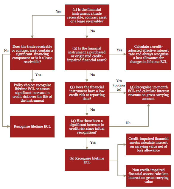
B. Impairment – During the global financial crisis, IASB realised that the incurred loss model in IAS 39 contributed to the delayed recognition of credit losses. To fix this issue, IASB introduced a forward-looking expected credit loss model. Under IFRS 9, the ECL model requires more timely recognition of credit losses. The new ECL Model was introduced through inception Stage 1, Stage 2 and Stage 3 whereby 12 Month ECL and Lifetime ECL are calculated under IFRS 9 compared to the incurred loss model of IAS 39.
| Stage | Definition | Impairment Calculation |
| Stage 1 | No significant credit risk increase | 12-month ECL |
| Stage 2 | Significant credit risk increase | Lifetime ECL |
| Stage 3 | Credit-impaired (default likely) | Lifetime ECL + interest on net carrying amount |
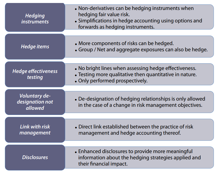
- C. Hedge accounting – The detailed rules under IAS 39 made hedge accounting impossible or very costly, even when the hedge had reflected economically rational risk management strategies. Thus, the rules for hedge accounting were less than perfect under IAS 39.
- There are still three types of hedging relationships: • Fair value hedges • Cash flow hedges • Hedges of net investments in foreign operations. High level Summary of Hedge Accounting changes are given below:
IFRS 9 vs. U.S. GAAP CECL
| Feature | IFRS 9 ECL | U.S. GAAP CECL |
| Time Horizon | 12-month (Stage 1) / Lifetime (Stages 2-3) | Lifetime ECL for all loans |
| Reversion Rules | Loans can move back to Stage 1 | No “stages,” but reversals allowed |
| Macroeconomic Adjustments | Required | Required |
IFRS 9 vs. IAS 39: Key Differences
- IFRS 9 reduced complexity by eliminating the “Available-for-Sale” and “Held-to-Maturity” categories.
- Introduced a more forward-looking impairment model (ECL), reducing procyclicality.
- Better aligned hedge accounting with risk management strategies.
| Feature | IAS 39 | IFRS 9 |
| Categories | Four categories: 1. Held-to-Maturity (HTM) 2. Loans & Receivables (L & R) 3. Fair Value Through Profit or Loss (FVTPL) 4. Available-for-Sale (AFS) | Three categories: 1. Amortized Cost 2. Fair Value Through OCI (FVOCI) 3. Fair Value Through Profit or Loss (FVTPL) + interest on net carrying amount |
| Basis for Classification | Based on management intent and instrument type. | Based on business model and cash flow characteristics (Solely Payments of Principal and Interest – SPPI). |
| Reclassification | Rarely allowed. | Permitted if business model changes. |
| Impairment Model | Incurred Loss Model (recognizes losses only after evidence of impairment). | Expected Credit Loss (ECL) Model (recognizes losses earlier, based on forward-looking estimates). |
| Stages | Not applicable. | Three stages of ECL Stage 1: 12-month ECL Stage 2: Lifetime ECL (credit risk increased significantly) Stage 3: Lifetime ECL (credit-impaired). |
| Hedging Approach | Highly rules-based, leading to mismatches. | More principle-based, allowing better alignment of risk management and accounting. |
| Hedging Eligibility | Strict criteria, often leading to inefficiencies. | More flexible, allowing non-derivatives as hedging instruments. |
| Hedging Effectiveness Testing | Required high effectiveness (80-125% range). | Less stringent, with a focus on economic relationship. |
IFRS 9 vs. Basel III: Key Differences
| Feature | IFRS 9 | Basel III |
| Primary Goal | Improve financial reporting by standardizing accounting for financial instruments | Strengthen bank capital, liquidity, and risk management to prevent financial crises |
| Nature | Accounting Standard Issued by IASB | Regulatory Framework Issued by BCBS |
| Key Focus | Expected Credit Loss (ECL) provisioning | Minimum capital requirements (CET1, Additional Tier 1, Tier 2) |
| Time Horizon | Lifetime ECL for impaired assets | 1-year risk horizon |
| Macroeconomic Impact | Forward-looking (incorporates economic forecasts) | Stress testing (fixed scenarios) |
| NPLs | Full lifetime ECL + interest adjustment | NPLs deducted from capital |
| Risk Weights | Not applicable | RWA determine capital requirements |
| PD | 12 Month PD-Stage 1 Lifetime PD- Stage 2 & Stage 3 | 12 Month PD |
| PD | PIT PD | TTC PD |
| Observation Period | No specific period | 5 Years- Retail 7 Years- Banks, Corporate, Sovereign |
| LGD/EAD | Best Estimate | Downturn Estimate |
| Capital Requirements | N/A | Sets minimum capital ratios (CET1, Tier 1, Total Capital) |
| Liquidity Standards | N/A | Introduces LCR and NSFR |
| Leverage Ratio | N/A | Limits excessive leverage via a non-risk-based leverage ratio |
| Floors | No prescribed floors | PD &LGD subject to floors |
| Classification & Measurement | Classifies financial assets into Amortized Cost, FVOCI, FVTPL | N/A |
| Impairment | Uses a forward looking ECL model | Uses an “Incurred Loss” model |
| Hedge Accounting | Provides more flexible hedge accounting rules | N/A |
| Capital Buffers | May increase loan loss provisions, affecting retained earnings | Requires capital conservation, countercyclical, and G-SIB buffers |
| Disclosures | Extensive footnote disclosures on financial instruments | Pillar 3 public disclosure requirements |
IFRS 9 Application
Challenges of IFRS 9 Implementation
While IFRS 9 improves financial reporting quality, its implementation posed several challenges for banks, insurers, and other financial institutions.
(1) Data Availability & Quality Challenge – IFRS 9 requires historical data, forward-looking macroeconomic data and probability-weighted scenarios to estimate ECL. Many Banks lacked sufficient historical loss data, especially for low-default portfolios. Poor data quality leads to unreliable ECL calculations and output.
(2) Complex Modeling & Judgment Challenge – IFRS 9 requires lifetime ECL for assets with significantly increased credit risk. (Stage 2 & Stage 3). Banks need to develop complex statistical models incorporating PD, LGD & EAD. High degree of management judgment in determining “significant increase in credit risk” (SICR) is required.
(3) Challenges in Macroeconomic Forecasting – IFRS 9 mandates incorporating forward-looking economic scenarios (GDP, employment, unemployment rates, CPI, HPI, Exchange Rate, Current Account, Budget Deficit, Public Debt, Sovereign Interest Rate, Bank Interest Rate and so on). Predicting future economic conditions (especially during crises like COVID-19) introduced volatility in ECL estimates.
(4) Increased Volatility in Profit & Loss (P&L – Earlier recognition of credit losses led to higher provisions and earnings volatility. Economic downturns result in higher ECL, further reducing reported profits.
(5) Business Model Assessment – IFRS 9 requires financial assets to be classified based on business model. Determining the primary business model is subjective, leading to inconsistencies.
(6) SPPI Test Challenges (Solely Payments of Principal & Interest) – Assets must pass the SPPI test to qualify for amortized cost or FVOCI. Complex instruments (e.g., convertible bonds, structured products) often failed SPPI, forcing FVTPL classification and increasing P&L volatility.
(7) Fair Value Measurement Issues – More assets are classified at FVTPL under IFRS 9, increasing reliance on fair value models. Illiquid instruments required Level 3 fair value inputs, raising valuation challenges.
(8) Challenges for Hedge Accounting Alignment with Risk Management – IFRS 9 allows more flexibility but requires documentation of risk management strategy. Many Banks struggled to align hedge accounting with their actual risk management practices.
(9) Challenges in Effectiveness Testing & Rebalancing of Hedge – Hedge effectiveness testing is less rigid but still requires ongoing monitoring. Moreover, changes in hedging relationships may require rebalancing, adding operational complexity.
(10) Challenges in System Upgrades & Integration – Legacy systems (designed for IAS 39) needed major upgrades to handle ECL calculations, New classification rules and Hedge accounting changes. Data silos and lack of integration made implementation difficult.
(11) Increased Compliance Costs – Banks and insurers incurred high costs for new software updation, Model and Scenario Development and training finance and risk teams.
(12) Transition Challenges for Restatement of Comparative Periods – IFRS 9 required retrospective application, meaning prior financial statements had to be restated. Many firms faced difficulties in recalculating opening balances.
(13) Capital & Regulatory Impact – Higher ECL provisions lead to reduced retained earnings, impacting regulatory capital ratios CET1 for banks.
(14) Missing Data Points – These are related to the instrument type; the credit risk ratings; the collateral type; the date of origination; the remaining term to maturity; the industry; the geographical location of the borrower; and the value of collateral relative to the commitment if it has an impact on the probability of default occurring (for example, non-recourse loans in some jurisdictions or loan-to-value ratios).
Calculation of Expected Credit Loss (ECL) Under IFRS 9
The Expected Credit Loss (ECL) model requires banks to estimate and provision for potential future credit losses before they occur, unlike the old IAS 39 “incurred loss” model. Here’s a step-by-step breakdown of how banks compute ECL:
1. Introduction to ECL Modelling -Expected Credit Loss (ECL) modelling is the quantitative framework banks and financial institutions use to estimate potential credit losses under IFRS 9. Unlike the old IAS 39 “incurred loss” approach, ECL is forward-looking, incorporating:
- Historical data
- Current economic conditions
- Reasonable forecasts
2. Key Components of ECL Modelling – The ECL model is built on three pillars:
A. Probability of Default (PD)
- Definition: Likelihood of a borrower will default within a given timeframe.
- Modelling Approaches:
- Statistical models (Logistic regression, survival analysis)
- Credit scoring (FICO scores, internal ratings)
- Machine learning (XGBoost, neural networks for non-linear patterns)
B. Loss Given Default (LGD)
- Definition: % of exposure lost after default (after recoveries).
- Calculation:
LGD = 1 – Recovery Rate
- Factors affecting LGD:
- Collateral quality
- Seniority of debt
- Legal recovery process
C. Exposure at Default (EAD)
- Definition: Amount at risk when default occurs.
- For loans = Outstanding principal + accrued interest
- For credit lines = Drawn amount + expected future drawdowns
ECL= PD×LGD×EAD
3. Step-by-Step ECL Calculation Process
Step 1: Data Preparation
- Collect 5+ years of historical default data
- Clean data (handle missing values, outliers)
- Segment portfolio (retail, corporate, SME)
Banks categorize loans/debt instruments into homogeneous groups (retail mortgages, corporate loans, credit cards) based on:
- Borrower type
- Collateral
- Risk rating
Step 2: Determine Probability of Default (PD)
- Internal models (using historical default data).
- External ratings (e.g., S&P, Moody’s).
- Forward-looking macroeconomic factors (GDP growth, unemployment, interest rates , inflation , exchange rate, public debt, HPI).
- For listed corporates: Use Merton’s structural model
- For retail: Behavioural scoring models
- Validation: Back-testing against actual defaults
Step 3: Estimate Loss Given Default (LGD)
- Collateral value (e.g., mortgages have lower LGD due to property backing).
- Recovery rates (how much the bank recovers post-default).
- Collateral haircuts: Apply discount to collateral value
- Workout LGD: Track actual recovery process
- Downturn LGD: Stress for recession scenarios
Step 4: Calculate Exposure at Default (EAD)
- For loans: Outstanding principal + accrued interest.
- For credit lines: Drawn amount + expected future drawdowns.
- Credit conversion factors (CCFs) for undrawn facilities
- Behavioural models for prepayments/revolvers
Step 5: Apply Time Horizon (12-Month vs. Lifetime ECL)
- Stage 1 (Performing loans) → 12-month ECL (short-term risk).
- Stage 2 (Significant risk increase) → Lifetime ECL (full loan term).
- Stage 3 (Impaired loans) → Lifetime ECL + adjusted interest.
Step 6: Scenario Analysis
- Base case
- Downturn scenario
- Severe but plausible scenario
Step 7: Advanced Modelling Techniques
| Technique | Application | Advantage |
| Survival Analysis | PD term structure | Accounts for time-to-default |
| Monte Carlo | Portfolio ECL | Captures correlation risk |
| Machine Learning | Non-linear relationships | Improves PD accuracy |
Step 8: Model Validation & Governance
- Discriminatory power testing: AUC-ROC > 0.7
- Calibration testing: Hosmer-Lemeshow test
- Stress testing: COVID-19 impact analysis
Corporate Loan ECL Calculation: Example
- PD: 2% (1-year), 8% (lifetime)
- LGD: 45%
- EAD: $10 million
12-month ECL = 2% × 45% × $10m = $90,000
Lifetime ECL = 8% × 45% × $10m = $360,000
Wholesale / Corporate IFRS 9 Model Building
The main activities that are involved in building a wholesale/corporate model are given below:
• Determine the client segmentation
• Define the targeted model structure (group / local model/ number of modules.)
• Define the input data and identify the candidate variables for the analysis – often split between quantitative factors (ROA, ROE, Debt Equity Ratio etc.) and qualitative factors (e.g. quality of the management, market share, market structure (monopoly v competitive), hurdles to entry).
• Definition of default, such as 30/60/90 DPD
• Perform data quality verification
• Define the historic data population for development and validation
• Development of subsequent modules:
o Univariate analysis
Definitions of the variables
Variables transformation
Categorization (if required)
Missing data analysis
Assessment of each variable – discriminatory power, stability, correlations
o Multivariate analyses
• Development of the joint model from separately developed modules
• Analyses of the prepared models, final model selection
• Pre-implementation tests
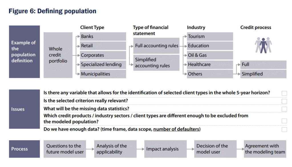
In terms of defining the population of data for Wholesale/Corporate IFRS 9 model, the following graphic provides a simplified guide to this process.
Retail IFRS 9 Model Building
(A) Credit Application Models for Individual candidate may include the followings:
• Socio-demographic variables: income, profession, region, age, marital status, education, employment type, employment duration etc.
• Relations with the Bank: length of the cooperation with the Bank, average amount of loans (or info on current account), product mix etc.
• Interactions between variables (complex variables) – like age and income, region and income etc.
• Variables based on credit bureau data, describing:
– Repayment history
– debt level, number of days past due
– History of loan origination (frequency, level of debt, loan types)
– History of queries to credit bureau.
(B) Behavioural Models for Individual candidate may include the followings:
• Behaviour on current accounts
• History on delinquency
• Level of exposure, exposure amount divided by exposure as at origination date
• Frequency of loan origination (how frequently the client takes new loans)
• Delinquency value to exposure value
• Usage of the available off-balance limit (in case of revolving products)
• Number, value, frequency or share of cash transactions and cashless transactions
• Repayment patterns for subsequent instalments
• History of cooperation with the bank
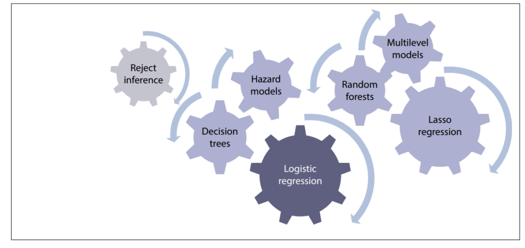
(C) Modelling Techniques for Retail Clients
It is difficult to select the perfect modeling technique for choosing a model for retail PD, LGD and EAD. It is advised to use several techniques or a combination of these. Final selection of the models is then based on its statistics and not on the assumptions of modeling techniques. Figure below provides a guide to some candidates for consideration:
Combination of Modelling Techniques
A typical number of steps in building a retail PD model for IFRS 9 is listed below. This is not meant to be exhaustive and is relative to IFRS 9 :
• Definition of the population to be covered by PD model (relation of the scoring models to PD models may vary in nature, as
o there are significant differences between the definition of ‘bad’ and ‘default’;
o segmentation for PD models is usually driven much more by IRB / IFRS 9 segmentation than the segmentation for scoring models
• Definition of additional data required for the preparation of PD model and data quality verification
• Development of a framework for calculating PD estimates based on historical default experience; use of statistical models for PD estimation for retail exposures (pool wise) and development of PD for retail pools
• Calculation of the Long Run Default Frequency (LRDF)
• Integration logic – matching the results from several scoring models into one PD
• Develop statistical process for derived variable creation and selection exercise; employ the calibration method (logistic regression or neural networks) and calibration of scores to LRDF
• Additional pooling factors for PD (if the model is to be based on pools)
• Calculation of the estimation error
• Pre-implementation validation: quality of the calibration, stability, concentration of the exposures in rating grades / pools.
• Finalize the model based on discussions and presentations made to the senior management
The process of creating an IFRS 9 Retail PD
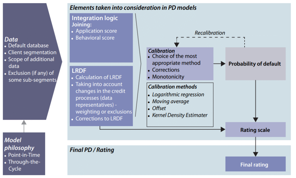
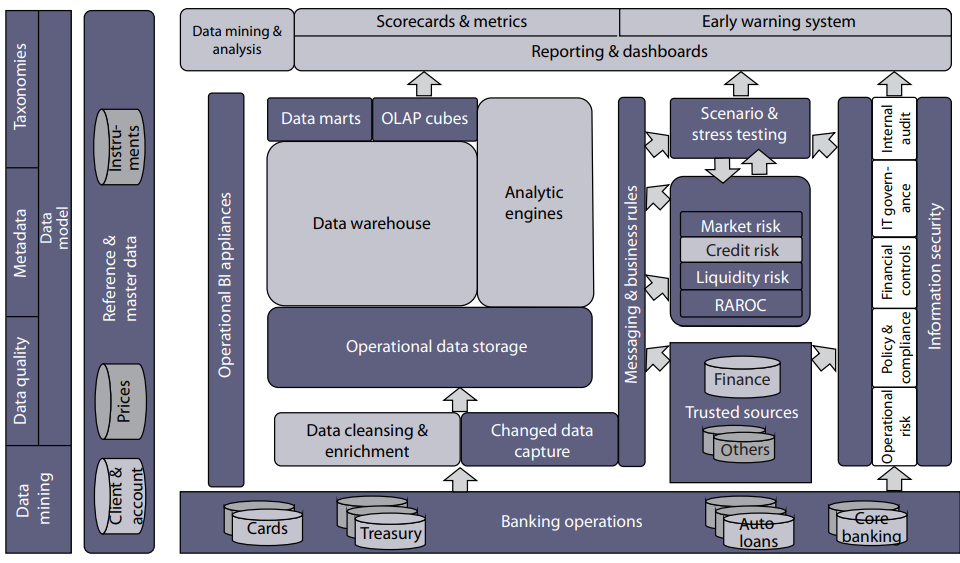
IT FRAMEWORK FOR IFRS 9
Point In Time PD: PIT PD is a forward- looking PD, taking into account the variations in economic cycle. PIT PD is calculated by using current macroeconomic variables such as GDP, Unemployment rate, Interest and Inflation rate, Housing price index, Exchange rate, Current Account and risk attributes of borrower. It does not contain adjustment for “prudence”. In essence PIT PD moves up as macro-economic conditions deteriorate and PIT PD moves down as macro-economic conditions improve. The PIT rating philosophy also implies that the resulting PIT PD will closely mimic observed default rates under ideal conditions.
Best Estimate PD: It means that PD estimates should be unbiased which means exclusion of optimism or conservatism (downturn) in estimation.
Through The Cycle PD: TTC PD includes only idiosyncratic factors and does not take into account the variations in economic cycle. As a result, TTC PD does not change with a change in macroeconomic factors. In such cases, the TTC PD shows little or no variation over the economic cycle and tends to deviate from the observed default rates only when the economy is at its peak or trough.
Hybrid PD: While the concept of pure PIT and TTC philosophy follower models or PDs is theoretical, in practice the PDs implied by such rating models tend to be at somewhere midway between PIT and TTC. Such PDs are called hybrid PIT-TTC PD.
Practical Python Implementation of an ECL model
Using synthetic data, covering PD, LGD, and EAD estimation with scenario analysis. Key Assumptions of This Model:
- PD Modelling
- Uses logistic regression with FICO, LTV, and DTI ratios
- AUC metric validates discriminatory power
- LGD Calculation
- Recovery rates based on collateral coverage
- Haircuts applied for under-collateralized loans
- Scenario Analysis
- 50% PD shock and 20% LGD shock for stress testing
- Caps to avoid unrealistic values (>99% PD, >95% LGD)
- Output Metrics
- Base case 12-month ECL
- Lifetime ECL (with 1.5x multiplier)
- Stressed ECL under adverse conditions
import numpy as np
import pandas as pd
from sklearn.linear_model import LogisticRegression
from sklearn.model_selection import train_test_split
from sklearn.metrics import roc_auc_score
# ======================
# 1. Synthetic Data Setup
# ======================
np.random.seed(42)
n_loans = 10_000
# Borrower features
data = pd.DataFrame({
‘FICO’: np.random.randint(500, 850, size=n_loans),
‘LTV’: np.random.uniform(0.5, 1.2, size=n_loans),
‘DebtToIncome’: np.random.uniform(0.1, 0.8, size=n_loans),
‘LoanAmount’: np.random.lognormal(10, 0.5, size=n_loans),
‘CollateralValue’: np.random.lognormal(11, 0.4, size=n_loans)
})
# Simulate defaults (PD)
data[‘Default’] = np.where(
(data[‘FICO’] < 600) &
(data[‘LTV’] > 0.8) &
(data[‘DebtToIncome’] > 0.5),
np.random.binomial(1, 0.8), # High-risk group
np.random.binomial(1, 0.05) # Low-risk group
)
# ======================
# 2. PD Model (Logistic Regression)
# ======================
X = data[[‘FICO’, ‘LTV’, ‘DebtToIncome’]]
y = data[‘Default’]
X_train, X_test, y_train, y_test = train_test_split(X, y, test_size=0.2)
model = LogisticRegression()
model.fit(X_train, y_train)
# Predict PDs
data[‘PD’] = model.predict_proba(X)[:, 1]
print(f”PD Model AUC: {roc_auc_score(y, data[‘PD’]):.2f}”)
# ======================
# 3. LGD Estimation
# ======================
data[‘RecoveryRate’] = np.where(
data[‘CollateralValue’] / data[‘LoanAmount’] > 1,
0.7, # Full collateral coverage
0.3 # Partial coverage
)
data[‘LGD’] = 1 – data[‘RecoveryRate’]
# ======================
# 4. EAD Calculation
# ======================
data[‘EAD’] = data[‘LoanAmount’] * 1.05 # Principal + 5% accrued interest
# ======================
# 5. ECL Calculation
# ======================
data[‘ECL_12m’] = data[‘PD’] * data[‘LGD’] * data[‘EAD’]
data[‘ECL_Lifetime’] = data[‘PD’] * 1.5 * data[‘LGD’] * data[‘EAD’] # Stress factor
# ======================
# 6. Scenario Analysis
# ======================
def apply_scenario(df, pd_shock=1.5, lgd_shock=1.2):
“””Apply macroeconomic stress scenario”””
stressed = df.copy()
stressed[‘PD’] = np.minimum(df[‘PD’] * pd_shock, 0.99) # Cap at 99%
stressed[‘LGD’] = np.minimum(df[‘LGD’] * lgd_shock, 0.95) # Cap at 95%
stressed[‘ECL_Stressed’] = stressed[‘PD’] * stressed[‘LGD’] * stressed[‘EAD’]
return stressed
stressed_data = apply_scenario(data)
# ======================
# 7. Portfolio Summary
# ======================
print(“\nPortfolio ECL Summary:”)
print(f”• Base Case 12m ECL: ${data[‘ECL_12m’].sum():,.0f}”)
print(f”• Lifetime ECL: ${data[‘ECL_Lifetime’].sum():,.0f}”)
print(f”• Stressed ECL: ${stressed_data[‘ECL_Stressed’].sum():,.0f}”)
# ======================
# 8. Visualization (requires matplotlib)
# ======================
import matplotlib.pyplot as plt
plt.figure(figsize=(10, 4))
plt.hist(data[‘PD’], bins=30, alpha=0.7, label=’PD Distribution’)
plt.axvline(data[‘PD’].mean(), color=’red’, linestyle=’dashed’, label=f’Mean PD: {data[“PD”].mean():.2%}’)
plt.title(‘Probability of Default Distribution’)
plt.xlabel(‘PD’)
plt.ylabel(‘Frequency’)
plt.legend()
plt.show()